この記事では、三角関数と双曲線関数、およびそれに関係の深い関数をまとめて記述する。
指数関数 、ベッセル関数 は個別ページを参照。
三角関数 [ ] 三角関数 (さんかくかんすう、英: trigonometric function 三角法 における、角 の大きさと線分 の長さの関係を記述する関数 の族 および、それらを拡張して得られる関数の総称である。三角関数 という呼び名は三角法に由来するもので、後述する単位円 を用いた定義に由来する呼び名として、円関数 (えんかんすう、英: circular function
三角関数には
sin
,
sec
,
tan
,
cos
,
csc
,
cot
{\displaystyle {\sin,\,\sec,\,\tan,\,\cos,\,\csc,\,\cot}}
の 6 つがあり、それぞれ正弦 (sin e) 、正割 (sec ant) 、正接 (tan gent) 、余弦 (cos ine) 、余割 (cosec ant) 、余接 (cot angent) を意味する。特に sin, cos は幾何学 的にも解析学 的にも良い性質を持っているので、様々な分野で用いられる。例えば波 や電気信号 などは正弦関数と余弦関数を組み合わせることで表現することができる。この事実はフーリエ級数 およびフーリエ変換 の理論として知られ、音声などの信号の合成や解析の手段として利用されている。他にもベクトル の外積 や内積 は正弦関数および余弦関数を用いて表すことができ、ベクトルを図形に対応づけることができる。初等的には、三角関数は実数 を変数 とする一変数関数として定義される。三角関数の変数の対応するものとしては、図形のなす角度や、物体の回転角、波や信号のような周期的 なものに対する位相 などが挙げられる。
三角関数に用いられる独特な記法として、三角関数の累乗 と逆関数 に関するものがある。通常、関数 f (x )(f (x ))2 = f (x )・f (x ) や (f (x ))−1 = 1 / f (x ) のように書くが、三角関数の累乗は sin2 x のように書かれることが多い。逆関数については通常の記法 (f −1 (x )sin−1 x などと表す(この文脈では従って、三角関数の逆数 は分数を用いて 1 / sin x (sin x )−1 などと表される)。文献あるいは著者によっては、通常の記法と三角関数に対する特殊な記法との混同を避けるため、三角関数の累乗を通常の関数と同様にすることがある。また、三角関数の逆関数として −1 と添え字する代わりに関数の頭に arc とつけることがある(たとえば sin の逆関数として sin−1 の代わりに arcsin を用いる)。
直角三角形による定義 [ ] ∠C を直角とする直角三角形ABC
直角三角形 において、1 つの鋭角の大きさが決まれば、三角形 の内角の和は 180° であることから他の 1 つの鋭角の大きさも決まり、3 辺の比も決まる。ゆえに、角度に対して辺比の値を与える関数を考えることができる。
∠C を直角とする直角三角形 ABC において、それぞれの辺の長さを AB = h , BC = a , CA = b と表す(図を参照)。∠A = θ に対して三角形の辺の比 h : a : b
{
sin
θ
=
a
h
sec
θ
=
h
b
=
1
cos
θ
tan
θ
=
a
b
=
sin
θ
cos
θ
{
cos
θ
=
b
h
cosec
θ
=
csc
θ
=
h
a
=
1
sin
θ
cot
θ
=
b
a
=
1
tan
θ
{\displaystyle \begin{align}
&\begin{cases}
\sin \theta = \frac{a}{h}\\
\sec \theta =\frac{h}{b} = \frac{1}{\cos \theta}\\
\tan \theta = \frac{a}{b} = \frac{\sin \theta}{\cos \theta}
\end{cases}\\
&\begin{cases}
\cos \theta = \frac{b}{h}\\
\operatorname{cosec}\theta = \csc \theta = \frac{h}{a} = \frac{1}{\sin \theta}\\
\cot \theta =\frac{b}{a} = \frac{1}{\tan \theta}
\end{cases}\end{align}}
という 6 つの値が定まる。それぞれ正弦 (sin e;正割 (sec ant;正接 (tan gent;余弦 (cos ine;余割 (cosec ant;余接 (cot angent;三角比 と呼ばれる。ただし cosec は長いので csc と略記することも多い。ある角 ∠A に対する余弦、余割、余接はその角 ∠A の余角 (co-angle) に対する正弦、正割、正接として定義される。
{
cos
θ
=
sin
(
90
∘
−
θ
)
=
sin
(
π
2
−
θ
)
csc
θ
=
sec
(
90
∘
−
θ
)
=
sec
(
π
2
−
θ
)
cot
θ
=
tan
(
90
∘
−
θ
)
=
tan
(
π
2
−
θ
)
{\displaystyle \begin{cases}
\cos \theta = \sin \left(90^\circ - \theta \right) = \sin \left(\frac{\pi}{2} - \theta \right)\\
\csc \theta = \sec \left(90^\circ - \theta \right) = \sec \left(\frac{\pi}{2} - \theta \right)\\
\cot \theta = \tan \left(90^\circ - \theta \right) = \tan \left(\frac{\pi}{2} - \theta \right)
\end{cases}}
三角比は平面三角法 に用いられ、巨大な物の大きさや遠方までの距離を計算する際の便利な道具となる。角度 θ の単位 は、通常度 またはラジアン である。
三角比、すなわち三角関数の直角三角形を用いた定義は、直角三角形の鋭角に対して定義されるため、その定義域は θ π / 2 θ = 90° (= π / 2 sec, tan が、θ = 0°(= 0)csc, cot がそれぞれ定義されない。これは分母となる辺の比の大きさが 0 になるためゼロ除算 が発生し、その除算自体が数学的に定義されないからである。一般の角度に対する三角関数を得るためには、三角関数について成り立つ何らかの定理を指針として、定義の拡張を行う必要がある。後述する単位円による定義 は初等幾何学におけるそのような拡張の例である。他に同等な方法として、正弦定理 や余弦定理 を用いる方法などがある。
単位円による定義 [ ] 単位円による、6つの三角関数が表す長さ
2 次元ユークリッド空間 R 2 単位円 {x (t )}2 + {y (t )}2 = 1 上の点を A = (x (t ), y (t )) とする。反時計回り を正の向きとして、原点と円周を結ぶ線分 OA と x 軸のなす角の大きさ ∠x OA を媒介変数 t として選ぶ。このとき実変数 t に対する三角関数は以下のように定義される。
sin
t
=
y
cos
t
=
x
tan
t
=
y
x
=
sin
t
cos
t
{\displaystyle \begin{align}
\sin t &= y\\
\cos t &= x\\
\tan t &= \frac{y}{x} = \frac{\sin t}{\cos t}
\end{align}}
これらは順に正弦関数 (sin e function) 、余弦関数 (cos ine function) 、正接関数 (tan gent function) と呼ばれる。さらにこれらの逆数 として以下の 3 つの関数が定義される。
csc
t
=
1
y
=
1
sin
t
sec
t
=
1
x
=
1
cos
t
cot
t
=
x
y
=
1
tan
t
{\displaystyle \begin{align}
\csc t &= \frac{1}{y} = \frac{1}{\sin t}\\
\sec t &= \frac{1}{x} = \frac{1}{\cos t}\\
\cot t &= \frac{x}{y} = \frac{1}{\tan t}
\end{align}}
これらは順に余割関数 (cosec ant function) 、正割関数 (sec ant function) 、余接関数 (cot angent function) と呼ばれ、sin, cos, tan と合わせて三角関数 と総称される。特に csc, sec, cot は割三角関数 (かつさんかくかんすう)と呼ばれることがある。
この定義は 0 < t < π / 2 の範囲では直角三角形による定義 と一致する。
級数による定義 [ ] 角度、辺の長さといった幾何学的な概念への依存を避けるため、また定義域 を複素数 に拡張するために、級数 を用いて定義することもできる。この定義は実数の範囲では単位円による定義と一致する。以下の級数は共に示される収束円内で収束 する。
sin
z
=
∑
n
=
0
∞
(
−
1
)
n
(
2
n
+
1
)
!
z
2
n
+
1
for all
z
,
cos
z
=
∑
n
=
0
∞
(
−
1
)
n
(
2
n
)
!
z
2
n
for all
z
,
tan
z
=
∑
n
=
1
∞
(
−
1
)
n
2
2
n
(
1
−
2
2
n
)
B
2
n
(
2
n
)
!
z
2
n
−
1
for
|
z
|
<
π
2
,
cot
z
=
∑
n
=
0
∞
(
−
1
)
n
2
2
n
B
2
n
(
2
n
)
!
z
2
n
−
1
for
0
<
|
z
|
<
π
,
sec
z
=
∑
n
=
0
∞
(
−
1
)
n
E
2
n
(
2
n
)
!
z
2
n
for
|
z
|
<
π
2
,
csc
z
=
∑
n
=
0
∞
(
−
1
)
n
(
2
−
2
2
n
)
B
2
n
(
2
n
)
!
z
2
n
−
1
for
0
<
|
z
|
<
π
.
{\displaystyle \begin{align}
\sin z &= \sum^{\infin}_{n=0} \frac{(-1)^n}{(2n+1)!} z^{2n+1}\quad \text{for all} \ z, \\
\cos z &= \sum^{\infin}_{n=0} \frac{(-1)^n}{(2n)!} z^{2n}\quad \text{for all} \ z, \\
\tan z &= \sum^{\infin}_{n=1} \frac{ (-1)^n 2^{2n} (1-2^{2n}) B_{2n}}{(2n)!} z^{2n-1}\quad \text{for} \ |z| < \frac{\pi}{2}, \\
\cot z &= \sum^{\infin}_{n=0} \frac{(-1)^n 2^{2n} B_{2n}}{(2n)!} z^{2n-1}\quad \text{for} \ 0 < |z| < \pi, \\
\sec z &= \sum^{\infin}_{n=0} \frac{(-1)^n E_{2n}}{(2n)!} z^{2n} \quad \text{for} \ |z|<\frac{\pi}{2}, \\
\csc z &= \sum^{\infin}_{n=0} \frac{(-1)^n (2-2^{2n}) B_{2n}}{(2n)!} z^{2n-1}\quad \text{for} \ 0 < |z|< \pi.
\end{align}}
微分方程式による定義 [ ] 実関数 f (x )常微分方程式 の初期値問題
f
″
(
x
)
=
−
f
(
x
)
,
f
(
0
)
=
1
,
f
′
(
0
)
=
0
{\displaystyle f''(x) = -f(x),\;f(0)=1,\;f'(0)=0}
(1 )
の解として cos x を定義し、sin x を −d (cos x )/dx として定義できる[1] [2] (1) g (x ) = f ' (x )
{
f
′
(
x
)
=
g
(
x
)
,
g
′
(
x
)
=
−
f
(
x
)
{\displaystyle \begin{cases}
f'(x) = g(x), \\
g'(x) = -f(x)
\end{cases}}
(2 )
および初期条件 f (0) = 1, g (0) = 0
他の定義 [ ] この他にも定積分による(逆三角関数を用いた)定義などが知られている[1] [3] [4]
周期性 [ ] sin x cos x
x 軸の正の部分となす角は
t
=
θ
+
2
π
n
(
0
≤
θ
<
2
π
,
n
∈
Z
)
{\displaystyle t=\theta +2\pi n\ (0\le \theta <2\pi ,n\isin \mathbb{Z} )}
と表すことができ、θ を偏角 、t を一般角 と言う。
一般角 t が 2π 進めば点 P(cos t , sin t ) は単位円上を 1 周し元の位置に戻る。従って、
cos
(
t
+
2
π
n
)
=
cos
t
sin
(
t
+
2
π
n
)
=
sin
t
{\displaystyle \begin{align}
\cos (t+2\pi n) &= \cos t \\
\sin (t+2\pi n) &= \sin t
\end{align}}
すなわち三角関数 cos, sin は周期 2π の周期関数 である。
ほぼ同様に、tan, cot は周期 π の周期関数、sec, csc は周期 2π の周期関数である。
三角関数のグラフ: Sine(青実線 )、 Cosine(緑実線 )、 Tangent(赤実線 )、 Cosecant(青点線 )、 Secant(緑点線 )、 Cotangent(赤点線 )
双曲線関数 [ ] 数学 において、双曲線関数 (そうきょくせんかんすう、英: hyperbolic function 三角関数 と類似の関数 で、標準形の双曲線 を媒介変数表示 するときなどに現れる。
概要 [ ] 斜線の領域の面積が /2 の時の単位円周上の座標が (cos , sin )
斜線の領域の面積が θ /2 の時の双曲線上の座標が(cosh θ, sinh θ )
三角関数は単位円周を用いて定義することができる。
以下、説明を簡単にするために第一象限(x ≧ 0、かつ、y ≧ 0)の話に限る。 単位円周上の点 A (cos θ, sin θ) と x 軸上の点 B (1, 0)、原点 O を考える。線分 AO 、 BO と弧 AB によって囲まれた領域 の面積は θ/2 である。
この性質を用いて逆に三角関数を定義することもできる。すなわち、単位円周上の点 A と x 軸上の点 B (1, 0)、 を取り、線分 AO 、BO と弧 AB によって囲まれた領域の面積が θ/2 であるとき、 A の座標を (cos θ, sin θ) として、三角関数を定義することができる。
単位円の定義式は
x
2
+
y
2
=
1
{\displaystyle x^2 + y^2 = 1}
であり、標準形の双曲線の定義式は y 2 の符号を変えただけの
x
2
−
y
2
=
1
{\displaystyle x^2 - y^2 = 1}
である。単位円の面積で三角関数を定義したのと同じように双曲線を用いて双曲線関数を定義することができる。
標準形の双曲線上の点 A と x 軸上の点 B (1, 0) を取り、線分 AO 、BO と双曲線の囲む領域の面積が θ/2 であるとき、 A の座標を (cosh θ, sinh θ) として、双曲線関数 cosh, sinh が定義される。
ちなみに、三角関数の定義に現れた θ は、弧度法 における角度に対応していたが、双曲線関数では角度には対応しない。
このように三角関数と双曲線関数は非常に似通った関数として定義され、いろいろな場面でその類似性が現れる。定義に双曲線を用いる関数を双曲線関数と呼ぶことにあわせて、定義に単位円を用いる三角関数の事を円関数 (circular function ) と呼ぶこともある。
定義 [ ] 一般に、双曲線関数は指数関数 e x
s
i
n
h
x
=
e
x
−
e
−
x
2
,
c
o
s
h
x
=
e
x
+
e
−
x
2
{\displaystyle {\rm sinh}\ x = {e^x - e^{-x} \over 2},\ \ {\rm cosh}\ x = {e^x + e^{-x} \over 2}}
と定義される。sinh, cosh をそれぞれ双曲線正弦 関数 (hyperbolic sine ; ハイパボリックサイン)、双曲線余弦 関数 (hyperbolic cosine ; ハイパボリックコサイン) と呼ぶ。他にも三角関数との類似で双曲線正接・余接関数
t
a
n
h
x
=
s
i
n
h
x
c
o
s
h
x
,
c
o
t
h
x
=
1
t
a
n
h
x
{\displaystyle {\rm tanh}\ x = {{\rm sinh}\ x \over {\rm cosh}\ x},\ \ {\rm coth}\ x = {1 \over {\rm tanh}\ x}}
や、双曲線正割・余割関数
s
e
c
h
x
=
1
c
o
s
h
x
,
c
o
s
e
c
h
x
=
1
s
i
n
h
x
{\displaystyle {\rm sech}\ x = {1 \over {\rm cosh}\ x},\ \ {\rm cosech}\ x = {1 \over {\rm sinh}\ x}}
なども定義できる。また、例えば cosh を cos hyp や
c
o
s
{\displaystyle \mathfrak{cos}}
このように定義された、双曲線正弦関数、双曲線余弦関数、双曲線正接関数、双曲線余接関数、双曲線正割関数、双曲線余割関数を総称して 双曲線関数 という。
指数関数 e x x を複素変数に拡張できるので、指数関数で定義されている双曲線関数自体も x を複素変数にとってもよい。
双曲線関数はいずれも名称が長いため、読むときは省略されることも多く sinh はシャイン あるいは シンチ 、cosh はコッシュ と読まれたりもする。
基本性質 [ ] sinh , cosh と tanh のグラフ。特にcosh x のグラフは懸垂線 として知られている。
csch , sech と coth のグラフ
指数関数 を偶関数 の部分と奇関数 の部分に分けた時、
e
x
=
cosh
x
+
sinh
x
{\displaystyle e^x = \cosh x + \sinh x}
e
−
x
=
cosh
x
−
sinh
x
{\displaystyle e^{-x} = \cosh x - \sinh x}
となり、偶関数部分が cosh x で、奇関数部分が sinh x であることが分かる。
また (cosh x , sinh x ) は、双曲線 x 2 − y 2 = 1 上の点であり
cosh
2
x
−
sinh
2
x
=
1
{\displaystyle \cosh^2 x - \sinh^2 x = 1}
逆三角関数 [ ] 数学 において、逆三角関数 (ぎゃくさんかくかんすう、英: inverse trigonometric function 、時折 cyclometric function [5] 定義域 を適切に制限した)三角関数 の逆関数 である。具体的には、それらは正弦 (sine) 、余弦 (cosine) 、正接 (tangent) 、余接 (cotangent) 、正割 (secant) 、余割 (cosecant) 関数の逆関数である。それらは角度の三角比の任意から角度を得るために使われる。逆三角関数は工学 、navigation 、物理学 、幾何学 において広く使われる。
表記 [ ] 逆三角関数に対して用いられるたくさんの表記がある。表記 sin−1 (x ) , cos−1 (x ) , tan−1 (x ) , etc. はしばしば使われるが、この慣習は関数の合成ではなく冪乗を意味する sin2 (x ) のような表現の一般的なセマンティクスと論理的には相反し、それゆえ乗法逆元 と合成的逆 の間の混乱を起こすかもしれない。三角関数の各逆数はそれ自身の名前を持っている、例えば cos(x )−1 =sec(x ) 、という事実によって混乱は幾分改善される。著者によっては別の慣習が使われる[6] Sin−1 (x ) , Cos−1 (x ) , etc. これは sin−1 (x ) , cos−1 (x ) , etc. によって表現されるべき乗法逆元との混乱を避ける。ところが語頭の大文字を主値を取ることを意味するために使う著者もいる。また別の慣習は接頭辞に arc- を用いることであり、右上の −1 の添え字の混乱は完全に解消される、例えば、arcsin (x ) , arccos (x ) , etc. この慣習は記事全体において用いられる。コンピュータプログラミング言語において逆三角関数は通常 asin, acos, atan と呼ばれる。
arc- 接頭辞の起源 [ ] ラジアン で測るとき、θ ラジアンの角度は長さが rθ の弧 (arc) に対応する。ただし r は円の半径である。従って、単位円 において、"コサインが x の arc" は "コサインが x である角度"と同じである、なぜならば単位円の弧長 はラジアンによって角度を測ったものと同じだからである[7]
基本的な性質 [ ] 主値 [ ] 6つの三角関数はいずれも単射 でないから、逆関数を持つように制限される。それゆえ逆関数の値域 はもとの関数の定義域の真の部分集合 である。
例えば、多価関数 の意味で関数 を用いて、平方根 関数 y = √ x y 2 = x y = arcsin(x )sin(y ) = x であるように定義される。sin(y ) = x であるような数 y は複数存在する; 例えば、sin(0) = 0 であるが、sin(π) = 0, sin(2π) = 0 , etc. でもある。ただ 1 つだけの値が望まれているとき、関数はその主枝 に制限される。この制限とともに、定義域の各 x に対して表現 arcsin(x ) はその主値 と呼ばれるただ 1 つの値だけを返す。これらの性質はすべての逆三角関数についても同様に当てはまる。
主逆関数は以下の表にリストされる。
名前
通常の表記
定義
実数を与える x の定義域
通常の主値の終域 ラジアン )
通常の主値の終域 度 )
arcsine y = arcsin x x = sin y −1 ≤ x ≤ 1 −π/2 ≤ y ≤ π/2 −90° ≤ y ≤ 90°
arccosine y = arccos x x = cos y −1 ≤ x ≤ 1 0 ≤ y ≤ π 0° ≤ y ≤ 180°
arctangent y = arctan x x = tan y すべての実数
−π/2 < y < π/2 −90° < y < 90°
arccotangent y = arccot x x = cot y すべての実数
0 < y < π 0° < y < 180°
arcsecant y = arcsec x x = sec y x ≤ −1 or 1 ≤ x 0 ≤ y < π/2 or π/2 < y ≤ π 0° ≤ y < 90° or 90° < y ≤ 180°
arccosecant y = arccsc x x = csc y x ≤ −1 or 1 ≤ x −π/2 ≤ y < 0 or 0 < y ≤ π/2 −90° ≤ y < 0° or 0° < y ≤ 90°
(注意: arcsecant 関数の終域を (0 ≤ y < π/2 or π ≤ y < 3π/2) と定義する著者もいる、なぜならば tangent 関数がこの定義域上非負だからである。これによっていくつかの計算がより首尾一貫したものになる。例えば、この終域を用いて、tan(arcsec(x )) = √ x 2 − 1 と表せる。一方で終域 (0 ≤ y < π/2 or π/2 < y ≤ π) を用いる場合、tan(arcsec(x )) = ± √ x 2 − 1 と書かねばならない、なぜならば tangent 関数は 0 ≤ y < π/2 上は負でないが π/2 < y ≤ π 上は正でないからである。類似の理由のため、同じ著者は arccosecant 関数の終域を (−π < y ≤ −π/2 or 0 < y ≤ π/2) と定義する。)
x が複素数 であることを許す場合、y の終域はその実部にのみ適用する。
応用 [ ] 一般の解 [ ] 各三角関数は引数の実部において周期的であり、2π の各区間において2度すべてのその値を取る。サインとコセカントは(k を整数として)周期を 2π k − π /2 で始め 2π k + π /2 で終わり、2π k + π /2 から 2π k + 3π /2 までは逆にする。コサインとセカントは周期を 2π k で始め 2π k + π で終わらせそれから 2π k + π から 2π k + 2π まで逆にする。タンジェントは周期を 2π k − π /2 から始め 2π k + π /2 で終わらせそれから 2π k + π /2 から 2π k + 3π /2 まで(前へ)繰り返す。コタンジェントは周期を 2π k で始め 2π k + π で終わらせそれから 2π k + π から 2π k + 2π まで(前へ)繰り返す。
この周期性は k を何か整数として一般の逆において反映される:
sin
(
y
)
=
x
⇔
y
=
arcsin
(
x
)
+
2
k
π
or
y
=
π
−
arcsin
(
x
)
+
2
k
π
{\displaystyle \sin(y) = x \ \Leftrightarrow\ y = \arcsin(x) + 2k\pi \text{ or } y = \pi - \arcsin(x) + 2k\pi}
1 つの方程式に書けば:
sin
(
y
)
=
x
⇔
y
=
(
−
1
)
k
arcsin
(
x
)
+
k
π
{\displaystyle \sin(y) = x \ \Leftrightarrow\ y = (-1)^k\arcsin(x) + k\pi}
cos
(
y
)
=
x
⇔
y
=
arccos
(
x
)
+
2
k
π
or
y
=
2
π
−
arccos
(
x
)
+
2
k
π
{\displaystyle \cos(y) = x \ \Leftrightarrow\ y = \arccos(x) + 2k\pi \text{ or } y = 2\pi - \arccos(x) + 2k\pi}
1 つの方程式に書けば:
cos
(
y
)
=
x
⇔
y
=
±
arccos
(
x
)
+
2
k
π
{\displaystyle \cos(y) = x \ \Leftrightarrow\ y = \pm\arccos(x) + 2k\pi}
tan
(
y
)
=
x
⇔
y
=
arctan
(
x
)
+
k
π
{\displaystyle \tan(y) = x \ \Leftrightarrow\ y = \arctan(x) + k\pi}
cot
(
y
)
=
x
⇔
y
=
arccot
(
x
)
+
k
π
{\displaystyle \cot(y)=x\ \Leftrightarrow \ y=\operatorname {arccot}(x)+k\pi }
sec
(
y
)
=
x
⇔
y
=
arcsec
(
x
)
+
2
k
π
or
y
=
2
π
−
arcsec
(
x
)
+
2
k
π
{\displaystyle \sec(y)=x\ \Leftrightarrow \ y=\operatorname {arcsec}(x)+2k\pi {\text{ or }}y=2\pi -\operatorname {arcsec}(x)+2k\pi }
csc
(
y
)
=
x
⇔
y
=
arccsc
(
x
)
+
2
k
π
or
y
=
π
−
arccsc
(
x
)
+
2
k
π
{\displaystyle \csc(y)=x\ \Leftrightarrow \ y=\operatorname {arccsc}(x)+2k\pi {\text{ or }}y=\pi -\operatorname {arccsc}(x)+2k\pi }
応用: 直角三角形の角度を見つけること [ ] 直角三角形。
逆三角関数は直角三角形 の残りの 2 つの角度を決定しようとするときに三角形の辺の長さが知られているときに有用である。例えば sin の直角三角形による定義を思い出すと
θ
=
arcsin
(
opposite
hypotenuse
)
{\displaystyle \theta = \arcsin \left( \frac{\text{opposite}}{\text{hypotenuse}} \right)}
が従う。しばしば、斜辺 (hypotenuse ) は未知であり arcsin や arccos を使う前にピタゴラスの定理 を使って計算される必要がある:a 2 + b 2 = h 2 h は 斜辺の長さである。アークタンジェントはこの状況で重宝する、なぜなら斜辺の長さは必要ないからだ。
θ
=
arctan
(
opposite
adjacent
)
.
{\displaystyle \theta = \arctan \left( \frac{\text{opposite}}{\text{adjacent}} \right).}
例えば、7 メートル行くと 3 メートル下がる屋根を考えよう。この屋根は水平線と角度 θ をなす。このとき θ は次のように計算できる:
θ
=
arctan
(
opposite
adjacent
)
=
arctan
(
rise
run
)
=
arctan
(
3
7
)
≈
23.2
∘
.
{\displaystyle \theta = \arctan \left(\frac{\text{opposite}}{\text{adjacent}} \right) = \arctan \left( \frac{\text{rise}}{\text{run}} \right) = \arctan \left( \frac{3}{7} \right) \approx 23.2^{\circ}.}
コンピュータサイエンスとエンジニアリングにおいて [ ] アークタンジェントの 2 引数の変種 [ ]
主要記事: atan2 atan2 関数は 2 つの引数を取り、与えられた y と x に対して y /x (−π, π] の範囲に定める。言い換えると、atan2(y , x ) は平面の正の x -軸とその上の点 (x , y ) の間の角度に反時計回り の角度(上半平面、y > 0y < 0atan2 関数は最初多くのコンピュータプログラミング言語において導入されたが、今日では他の科学や工学の分野においても一般的に用いられている。
atan2 は標準的な arctan 、すなわち終域を (−π/2, π/2) に持つ、を用いて次のように表現できる:
atan2
(
y
,
x
)
=
{
arctan
(
y
x
)
x
>
0
arctan
(
y
x
)
+
π
y
≥
0
,
x
<
0
arctan
(
y
x
)
−
π
y
<
0
,
x
<
0
π
2
y
>
0
,
x
=
0
−
π
2
y
<
0
,
x
=
0
undefined
y
=
0
,
x
=
0
{\displaystyle \operatorname{atan2}(y, x) = \begin{cases}
\arctan(\frac y x) & \qquad x > 0 \\
\arctan(\frac y x) + \pi & \qquad y \ge 0 , x < 0 \\
\arctan(\frac y x) - \pi & \qquad y < 0 , x < 0 \\
\frac{\pi}{2} & \qquad y > 0 , x = 0 \\
-\frac{\pi}{2} & \qquad y < 0 , x = 0 \\
\text{undefined} & \qquad y = 0, x = 0
\end{cases}}
それはまた複素数 x + iy 偏角 の主値 にも等しい。
この関数はタンジェント半角公式を用いて次のようにも定義できる: x > 0y ≠ 0
atan2
(
y
,
x
)
=
2
arctan
y
x
2
+
y
2
+
x
{\displaystyle \operatorname{atan2}(y, x)=2\arctan \frac{y}{\sqrt{x^2 + y^2} + x} }
しかしながらこれは x ≤ 0y = 0
上の引数の順序 (y , x ) は最も一般的のようであり、特にC言語のようなISO規格において用いられるが、少数の著者は逆の慣習 (x , y ) を用いているため、注意が必要である。これらのバリエーションは atan2 に詳しい。
x, y 共に 0 の場合、インテルの CPU の FPATAN 命令、Javaプラットフォーム、.NET Framework などは下記ルールに従っている。
atan2(+0, +0) = +0
atan2(+0, −0) = +π
atan2(−0, +0) = −0
atan2(−0, −0) = −π 位置パラメータを伴うアークタンジェント関数 [ ] 多くの応用において[どれ? 方程式 x = tan y y は与えられた値 −∞ < η < ∞ にできるだけ近い値を取るべきである。適切な解はパラメータ修正アークタンジェント関数
y
=
arctan
η
x
:=
arctan
x
+
π
⋅
rni
η
−
arctan
x
π
{\displaystyle y=\arctan_\eta x:=\arctan x+\pi\cdot\operatorname{rni}\frac{\eta-\arctan x}{\pi} \, }
によって得られる。丸め関数
rni
{\displaystyle \operatorname{rni}}
(r ound to the n earest i nteger) 。
実際的考慮 [ ] 0 と π の近くの角度に対して、アークコサインは ill-conditioned であり、計算機において角度計算の実装に用いると精度が落ちてしまう(桁数の制限のため)。同様に、アークサインは −π/2 と π/2 の近くの角度に対して精度が低い。すべての角度に対して十分な精度を達成するには、実装ではアークタンジェントあるいは atan2 を使うべきである。
逆双曲線関数 [ ] 関数 artanh のグラフ
逆双曲線関数 (ぎゃくそうきょくせんかんすう、英語: inverse hyperbolic functions )は、数学 において与えられた双曲線関数 の値に対応して双曲角 を与える関数 。双曲角の大きさは双曲線 x y = 1に対応する双曲的扇形 の面積 に等しく、単位円 の扇形 の面積は対応する中心角 の2分の1 である。一部の研究者は逆双曲線関数のことを、双曲角を明確に理解するため「面積関数」(英語: area function )と呼ぶ。
逆双曲線関数を表す略記法 arsinh やarcosh とは異なる略記法として、arcsinh やarccosh などが本来誤表記であるにも関わらす良く使用されるのだが、接頭辞 arc はarcus (弓 )の省略形であり、接頭辞ar はarea の省略形である[8] [9] [10] 計算機科学 の分野では、しばしばasinh という省略形を用いる。累乗 を表す上付き文字−1と誤解しないように注意を払う必要があるという事実にもかかわらず、sinh−1 (x ), cosh−1 (x ), などの略記も用いられる。また、cosh−1 (x ) とcosh(x )−1 は似て非なるものである。
対数表現 [ ] 演算子 は複素数平面 で次のように定義される。
arsinh
z
=
ln
(
z
+
z
2
+
1
)
arcosh
z
=
ln
(
z
+
z
+
1
z
−
1
)
artanh
z
=
1
2
ln
(
1
+
z
1
−
z
)
arcoth
z
=
1
2
ln
(
z
+
1
z
−
1
)
arcsch
z
=
ln
(
1
z
+
1
z
2
+
1
)
arsech
z
=
ln
(
1
z
+
1
z
+
1
1
z
−
1
)
{\displaystyle
\begin{align}
\operatorname{arsinh}\, z &= \ln(z + \sqrt{z^2 + 1} \,)
\\[2.5ex]
\operatorname{arcosh}\, z &= \ln(z + \sqrt{z+1} \sqrt{z-1} \,)
\\[1.5ex]
\operatorname{artanh}\, z &= \tfrac12\ln\left(\frac{1+z}{1-z}\right)
\\
\operatorname{arcoth}\, z &= \tfrac12\ln\left(\frac{z+1}{z-1}\right)
\\
\operatorname{arcsch}\, z &= \ln\left( \frac{1}{z} + \sqrt{ \frac{1}{z^2} +1 } \,\right)
\\
\operatorname{arsech}\, z &= \ln\left( \frac{1}{z} + \sqrt{ \frac{1}{z} + 1 } \, \sqrt{ \frac{1}{z} -1 } \,\right)
\end{align}
}
上記の平方根 は正の平方根であり、対数関数 は複素対数である。実数の引数 、例えばz = xは実数値を返すが、一定の簡素化を行うことが可能であり、例えば
x
+
1
x
−
1
=
x
2
−
1
{\displaystyle \sqrt{x+1}\sqrt{x-1}=\sqrt{x^2-1}}
グーデルマン関数 [ ] グーデルマン関数 (グーデルマンかんすう、英語: Gudermannian function 、ドイツ語 : Gudermannfunktion )は、クリストフ・グーデルマン(1798–1852)にちなんで命名された、複素数 を用いない三角関数及び双曲線関数と関係する関数 。
定義 [ ] グーデルマン関数とその漸近線 y = ±π/2を青色で示した図
定義は以下のとおりである。
g
d
x
=
∫
0
x
d
t
cosh
t
=
arcsin
(
tanh
x
)
=
a
r
c
t
a
n
(
sinh
x
)
=
2
arctan
[
tanh
(
1
2
x
)
]
=
2
arctan
(
e
x
)
−
1
2
π
.
{\displaystyle \begin{align}{\rm{gd}}\,x&=\int_0^x\frac{dt}{\cosh t} \\[8pt]
&=\arcsin\left(\tanh x \right)
=\mathrm{arctan}\left(\sinh x \right) \\[8pt]
&=2\arctan\left[\tanh\left(\frac{1}{2}x\right)\right]
=2\arctan(e^x)-\frac{1}{2}\pi.
\end{align}\,\!}
グーデルマン関数と関連する公式 の中には、定義として全く運用できないものがある。例えば、実数x について、
arccos
s
e
c
h
x
=
|
g
d
x
|
=
arcsec
(
cosh
x
)
{\displaystyle \arccos \mathrm {sech} \,x=\vert \mathrm {gd} \,x\vert =\operatorname {arcsec}(\cosh x)}
歴史 [ ] この関数は、ヨハン・ハインリッヒ・ランベルトによって1760年代に双曲線関数と同じ頃に紹介された。彼はそれを「超越角」(transcendent angle )と呼び、アーサー・ケイリーが1862年に、1830年代のグーデルマンによる特殊関数 の理論の功績にちなんで「グーデルマン関数」と呼ぶことを提案するまで、様々な名称で呼ばれてきた[11] sinh とcosh (同書では
S
i
n
{\displaystyle \mathfrak{Sin}}
C
o
s
{\displaystyle \mathfrak{Cos}}
Theorie der potenzial- oder cyklisch-hyperbolischen functionen
グーデルマン関数を表す記号gd は、Philosophical Magazine [12] gd. u を用いたのが始まりである。ここで、
u
=
∫
0
ϕ
sec
t
d
t
=
ln
tan
(
1
4
π
+
1
2
ϕ
)
{\displaystyle u = \int_0^\phi \sec t \,dt = \ln\tan\left(\frac{1}{4}\pi+\frac{1}{2}\phi\right)}
であり、超越の定義を次のように示した。
gd
u
=
i
−
1
ln
tan
(
1
4
π
+
1
2
u
i
)
{\displaystyle \operatorname{gd} \,u = i^{-1}\ln\tan\left(\frac{1}{4}\pi+\frac{1}{2}ui\right)}
よって、それはu の実関数 であることが即座に見いだされる。
適用 [ ] 地球を真球 と見立てたとき、メルカトル図法 による投影面上における、赤道 からの緯線 距離についてのグーデルマン関数の関数値は、子午線弧 長、すなわち実際の地球上の緯度 に相当する。ガウス・クリューゲル図法 による地図投影 においては、座標換算の中間変数として用いられる正角緯度 の導入時においてもグーデルマン関数が現れる[13]
また、グーデルマン関数は、倒立振子(とうりつしんし、Inverted pendulum )の非周期解に現れる[14]
逆グーデルマン関数 [ ] グーデルマン関数の逆関数
グーデルマン関数の逆関数 (逆グーデルマン関数又はランベルト関数と称する)は、区間
(
−
π
/
2
,
π
/
2
)
{\displaystyle \left(-\pi/2, \pi/2\right)}
gd
−
1
x
=
∫
0
x
d
t
cos
t
=
ln
|
1
+
sin
x
cos
x
|
=
1
2
ln
|
1
+
sin
x
1
−
sin
x
|
=
ln
|
tan
x
+
sec
x
|
=
ln
|
tan
(
1
4
π
+
1
2
x
)
|
=
a
r
t
a
n
h
(
sin
x
)
=
a
r
s
i
n
h
(
tan
x
)
.
{\displaystyle
\begin{align}
\operatorname{gd}^{-1}\,x & = \int_0^x\frac{dt}{\cos t} \\[8pt]
& = \ln\left| \frac{1 + \sin x}{\cos x} \right| = \frac{1}{2}\ln \left| \frac{1 + \sin x}{1 - \sin x} \right| \\[8pt]
& = \ln\left| \tan x +\sec x \right| = \ln \left| \tan\left(\frac{1}{4}\pi + \frac{1}{2}x\right) \right| \\[8pt]
& = \mathrm{artanh}\,(\sin x) = \mathrm{arsinh}\,(\tan x).
\end{align}
}
sinc関数 [ ] 正規化sinc(青) と非正規化sinc(赤)。−6π ≤ x ≤ 6π
sinc 関数 (ジンクかんすう、シンクかんすう)は、正弦関数をその変数で割って得られる初等関数 である。sinc(x ), Sinc(x ), sinc x などで表される。
定義 [ ] sinc 関数は、正規化 sinc 関数と非正規化 sinc 関数という名で区別される、2種類の定義を持つ。
デジタル信号処理 などでは、次の正規化 sinc 関数 (標本化関数 ともいう)が普通である。
s
i
n
c
(
x
)
=
sin
π
x
π
x
.
{\displaystyle \mathrm{sinc}(x) = \frac{\sin \pi x}{\pi x}.}
数学 では、次の歴史的な非正規化 sinc 関数 が使われる。
s
i
n
c
(
x
)
=
sin
x
x
.
{\displaystyle \mathrm{sinc}(x) = \frac{\sin x}{x}.}
いずれの場合も、可除特異点である 0 での値が必要であればしばしば明示的に sinc(0) = 1 が定義として与えられる。sinc 関数はいたるところ解析的 である。
sinc 関数は カーディナル・サイン (cardinal sine) とも呼ばれ、"sinc" (英語発音: [ˈsɪŋk] sinus cardinalis を短縮したものである。
sinc関数の性質 [ ] 特にことわらないかぎり、正規化sinc関数について述べる。非正規化sinc関数は、スケールファクタ
π
{\displaystyle \pi }
x
←
x
/
π
{\displaystyle x \leftarrow x / \pi \,}
直交性 [ ]
∫
−
∞
∞
s
i
n
c
(
x
−
i
)
s
i
n
c
(
x
−
j
)
d
x
=
δ
i
j
,
if
i
,
j
∈
Z
{\displaystyle \int_{-\infty}^{\infty} \mathrm{sinc}(x-i)\mathrm{sinc}(x-j) \, dx = \delta_{ij}, \mbox{ if } i, j \in \mathbb{Z}}
信号処理への応用 [ ] さまざまな用途が考えられるが、コンパクト・サポート でない(非0の値が有限区間に限定されていない)ため、非常に多くの計算量を要することが多い。有限長で計算をうち切らなければならないことも多く、無限長では生じない問題が発生することもある。概して、理論的背景やシミュレーションにとどまることが多い。
直交性と ±∞ での収束性から、直交ウェーブレット変換 の基底 に用いる。ただし、コンパクト・サポートでないため、計算量が O(N 2 )(ランダウの記号 )で増える。これは、コンパクト・サポートな基底だと計算量が O (N ) であることに比べ、大きなデメリットである。
sinc 関数のフーリエ変換が矩形関数であることから、リサンプリング や内挿 の補間カーネル (低域通過フィルタ )に用いる。無限系列の信号に対しては、sinc 関数は理想的な補間カーネルである。しかし、コンパクト・サポートでないことが実際の有限長の信号を処理する際には問題となるため、実際の信号処理では、sinc 関数に似たコンパクト・サポート関数である、3次畳み込み関数や、ランツォシュ・フィルタ(Lanczosフィルタ)などが使われることが多い。
矩形関数のフーリエ変換がsinc 関数であることから、sinc 関数を使えば、理想的なD/A変換 ができる。ただしこれは、重要な概念ではあるが、実際にこのやりかたで D/A 変換がなされるわけではない。
その他の関数 [ ] 平行角関数 [ ] 数式
π
/
2
−
g
d
x
{\displaystyle \pi/2 - \mathrm{gd}\,x}
双曲幾何学 において、平行角 関数を定義する。
haversine 半正矢関数 [ ]
hav
x
=
d
e
f
1
2
(
1
−
cos
x
)
=
sin
2
x
2
{\displaystyle \operatorname{hav}x \ \overset{\underset{\mathrm{def}}{}}{=} \ \frac{1}{2}(1-\cos x) = \sin ^2\frac{x}{2} \!}
で定義される半正矢関数
hav
(
)
{\displaystyle \operatorname{hav}() }
hav
(
−
x
)
=
hav
x
{\displaystyle \operatorname{hav}(-x) = \operatorname{hav}x }
cos
x
=
1
−
2
hav
x
{\displaystyle \cos x = 1-2\operatorname{hav}x \!}
1
−
2
hav
a
=
cos
b
cos
c
+
sin
b
sin
c
(
1
−
2
hav
A
)
{\displaystyle 1-2\operatorname{hav}a = \cos b \cos c + \sin b \sin c (1-2\operatorname{hav}A) \!}
より
hav
a
=
hav
(
b
−
c
)
+
sin
b
sin
c
hav
A
{\displaystyle \operatorname{hav}a\ = \operatorname{hav}(b-c)+\sin b \sin c\ \operatorname{hav} A\!
}
となる。
古い関数 [ ] 単位円と角 θ に対する三角関数の関係。
三角関数から求められる versine, coversine, haversine, exsecant などの各関数は、かつて測量 などに用いられた。例えば haversine は球面上の2点の距離を求めるのに使用された。haversineを使用すると関数表の表をひく回数を減らすことができるからである。(参考:球面三角法 ) 今日ではコンピュータの発達により、これらの関数はほとんど使用されない。
versine と coversine は日本語では「正矢」「余矢」と呼ばれ、三角関数とともに八線表 として1つの数表にまとめられていた。
名前
表記
値
versed sine, versine
versin
θ
{\displaystyle \operatorname{versin}\theta}
vers
θ
{\displaystyle \operatorname{vers}\theta}
ver
θ
{\displaystyle \operatorname{ver}\theta}
1
−
cos
θ
{\displaystyle 1 - \cos\theta\!}
versed cosine, vercosine
vercosin
θ
{\displaystyle \operatorname{vercosin}\theta}
1
+
cos
θ
{\displaystyle 1 + \cos\theta\!}
coversed sine, coversine
coversin
θ
{\displaystyle \operatorname{coversin}\theta}
cvs
θ
{\displaystyle \operatorname{cvs}\theta}
1
−
sin
θ
{\displaystyle 1 - \sin\theta\!}
coversed cosine, covercosine
covercosin
θ
{\displaystyle \operatorname{covercosin}\theta}
1
+
sin
θ
{\displaystyle 1 + \sin\theta\!}
half versed sine, haversine
haversin
θ
{\displaystyle \operatorname{haversin}\theta}
1
−
cos
θ
2
{\displaystyle \frac{1 - \cos \theta}{2}}
half versed cosine, havercosine
havercosin
θ
{\displaystyle \operatorname{havercosin}\theta}
1
+
cos
θ
2
{\displaystyle \frac{1 + \cos \theta}{2}}
half coversed sine, hacoversine
hacoversin
θ
{\displaystyle \operatorname{hacoversin}\theta}
1
−
sin
θ
2
{\displaystyle \frac{1 - \sin \theta}{2}}
half coversed cosine, hacovercosine
hacovercosin
θ
{\displaystyle \operatorname{hacovercosin}\theta}
1
+
sin
θ
2
{\displaystyle \frac{1 + \sin \theta}{2}}
exterior secant, exsecant
exsec
θ
{\displaystyle \operatorname{exsec}\theta}
sec
θ
−
1
{\displaystyle \sec\theta - 1\!}
exterior cosecant, excosecant
excsc
θ
{\displaystyle \operatorname{excsc}\theta}
csc
θ
−
1
{\displaystyle \csc\theta - 1\!}
chord弦 の長さ)
crd
θ
{\displaystyle \operatorname{crd}\theta}
2
sin
θ
2
{\displaystyle 2\sin\frac{\theta}{2}}
複素平面 [ ] 三角関数 [ ] exp z , cos z , sin z の級数による定義 から、オイラーの公式 exp (iz ) = cos z + i sin z を導くことができる。この公式から下記の 2 つの等式
exp
(
i
z
)
=
e
i
z
=
cos
z
+
i
sin
z
,
exp
(
−
i
z
)
=
e
−
i
z
=
cos
z
−
i
sin
z
{\displaystyle \begin{align}
\exp(iz) &= e^{iz} = \cos z + i \sin z,\\
\exp(-iz) &= e^{-iz} = \cos z - i \sin z
\end{align}}
が得られるから、これを連立させて解くことにより、正弦関数・余弦関数の指数関数 を用いた表現が可能となる。即ち、
cos
z
=
e
i
z
+
e
−
i
z
2
,
sin
z
=
e
i
z
−
e
−
i
z
2
i
{\displaystyle \begin{align}
\cos z &= \frac{e^{iz} + e^{-iz}}{2} ,\\
\sin z &= \frac{e^{iz} - e^{-iz}}{2i}
\end{align}}
が成り立つ。この事実により、級数によらずこの等式をもって複素変数の正弦・余弦関数の定義とすることもある。また、
cos
(
i
z
)
=
e
−
z
+
e
z
2
=
cosh
z
,
sin
(
i
z
)
=
e
−
z
−
e
z
2
i
=
i
sinh
z
{\displaystyle \begin{align}
\cos(iz) &= \frac{e^{-z} +e^z}{2} = \cosh z, \\
\sin(iz) &= \frac{e^{-z} -e^z}{2i} = i\sinh z
\end{align}}
が成り立つ。ここで cosh z , sinh z は双曲線関数 を表す。この等式は三角関数と双曲線関数の関係式と捉えることもできる。複素数 z を z = x + iy (x , y ∈ R )
cos
z
=
cos
(
x
+
i
y
)
=
cos
x
cosh
y
−
i
sin
x
sinh
y
,
sin
z
=
sin
(
x
+
i
y
)
=
sin
x
cosh
y
+
i
cos
x
sinh
y
{\displaystyle \begin{align}
\cos z &= \cos(x + iy) = \cos x \cosh y - i \sin x \sinh y, \\
\sin z &= \sin(x + iy) = \sin x \cosh y + i \cos x \sinh y
\end{align}}
が成り立つ。
他の三角関数は csc z = 1 / sin z , sec z = 1 / cos z , tan z = sin z / cos z , cot z = cos z / sin z によって定義できる。
逆三角関数 [ ] 逆三角関数は解析関数 であるから、実数直線から複素平面に拡張することができる。その結果は複数のシートと分岐点 を持つ関数になる。拡張を定義する 1 つの可能な方法は:
arctan
z
=
∫
0
z
d
x
1
+
x
2
z
≠
−
i
,
+
i
{\displaystyle \arctan z = \int_0^z \frac{d x}{1 + x^2} \quad z \neq -i, +i \,}
ただし −i と +i の真の間にない虚軸の部分は主シートと他のシートの間の cut である;
arcsin
z
=
arctan
z
1
−
z
2
z
≠
−
1
,
+
1
{\displaystyle \arcsin z = \arctan \frac{z}{\sqrt{1 - z^2}} \quad z \neq -1, +1 \,}
ただし(平方根関数は負の実軸に沿って cut を持ち)−1 と +1 の真の間にない実軸の部分は arcsin の主シートと他のシートの間の cut である;
arccos
z
=
π
2
−
arcsin
z
z
≠
−
1
,
+
1
{\displaystyle \arccos z = \frac{\pi}{2} - \arcsin z \quad z \neq -1, +1 \,}
これは arcsin と同じ cut を持つ;
arccot
z
=
π
2
−
arctan
z
z
≠
−
i
,
+
i
{\displaystyle \operatorname {arccot} z={\frac {\pi }{2}}-\arctan z\quad z\neq -i,+i\,}
これは arctan と同じ cut を持つ;
arcsec
z
=
arccos
1
z
z
≠
−
1
,
0
,
+
1
{\displaystyle \operatorname {arcsec} z=\arccos {\frac {1}{z}}\quad z\neq -1,0,+1\,}
ただし −1 と +1 の両端を含む間の実軸の部分は arcsec の主シートと他のシートの間の cut である;
arccsc
z
=
arcsin
1
z
z
≠
−
1
,
0
,
+
1
{\displaystyle \operatorname {arccsc} z=\arcsin {\frac {1}{z}}\quad z\neq -1,0,+1\,}
これは arcsec と同じ cut を持つ。
対数を使った形 [ ] これらの関数は複素対数関数 を使って表現することもできる。これらの関数の対数表現は三角関数の指数関数による表示を経由して初等的な証明が与えられ、その定義域 を複素平面 に自然に拡張する。
arcsin
x
=
−
i
log
(
i
x
+
1
−
x
2
)
=
arccsc
1
x
arccos
x
=
i
log
(
x
−
i
1
−
x
2
)
=
π
2
+
i
log
(
i
x
+
1
−
x
2
)
=
π
2
−
arcsin
x
=
arcsec
1
x
arctan
x
=
1
2
i
(
log
(
1
−
i
x
)
−
log
(
1
+
i
x
)
)
=
arccot
1
x
arccot
x
=
1
2
i
(
log
(
1
−
i
x
)
−
log
(
1
+
i
x
)
)
=
arctan
1
x
arcsec
x
=
−
i
log
(
i
1
−
1
x
2
+
1
x
)
=
i
log
(
1
−
1
x
2
+
i
x
)
+
π
2
=
π
2
−
arccsc
x
=
arccos
1
x
arccsc
x
=
−
i
log
(
1
−
1
x
2
+
i
x
)
=
arcsin
1
x
{\displaystyle {\begin{aligned}\arcsin x&{}=-i\,\log \left(i\,x+{\sqrt {1-x^{2}}}\right)&{}=\operatorname {arccsc} {\frac {1}{x}}\\[10pt]\arccos x&{}=i\,\log \left(x-i\,{\sqrt {1-x^{2}}}\right)={\frac {\pi }{2}}\,+i\log \left(i\,x+{\sqrt {1-x^{2}}}\right)={\frac {\pi }{2}}-\arcsin x&{}=\operatorname {arcsec} {\frac {1}{x}}\\[10pt]\arctan x&{}={\frac {1}{2}}\,i\left(\log \left(1-i\,x\right)-\log \left(1+i\,x\right)\right)&{}=\operatorname {arccot} {\frac {1}{x}}\\[10pt]\operatorname {arccot} x&{}={\frac {1}{2}}\,i\left(\log \left(1-{\frac {i}{x}}\right)-\log \left(1+{\frac {i}{x}}\right)\right)&{}=\arctan {\frac {1}{x}}\\[10pt]\operatorname {arcsec} x&{}=-i\,\log \left(i\,{\sqrt {1-{\frac {1}{x^{2}}}}}+{\frac {1}{x}}\right)=i\,\log \left({\sqrt {1-{\frac {1}{x^{2}}}}}+{\frac {i}{x}}\right)+{\frac {\pi }{2}}={\frac {\pi }{2}}-\operatorname {arccsc} x&{}=\arccos {\frac {1}{x}}\\[10pt]\operatorname {arccsc} x&{}=-i\,\log \left({\sqrt {1-{\frac {1}{x^{2}}}}}+{\frac {i}{x}}\right)&{}=\arcsin {\frac {1}{x}}\end{aligned}}}
ここで注意しておきたい事は、複素対数関数における主値は、複素数の偏角部分 arg の主値の取り方に依存して決まる事である。それ故に、ここで示した対数表現における主値は、複素対数関数の主値を基準にすると、逆三角関数の主値 で述べた通常の主値と一致しない場合がある事に注意する必要がある。一致させたい場合は、対数部の位相をずらす事で対応できる。若し文献により異なる対数表現が与えられている樣な場合には、主値の範囲を異なる範囲で取る場合であると考えられるので、目的に応じて対数部の位相をずらす必要がある。
証明例 [ ]
θ
=
arcsin
x
{\displaystyle \theta = \arcsin x }
sin
(
θ
)
=
sin
(
arcsin
x
)
{\displaystyle \sin(\theta) = \sin(\arcsin x) }
sin
(
θ
)
=
x
{\displaystyle \sin(\theta) = x }
サインの指数関数による定義
e
i
ϕ
−
e
−
i
ϕ
2
i
=
sin
(
ϕ
)
{\displaystyle \frac{e^{i\phi} - e^{-i\phi}}{2i} = \sin(\phi) }
を用いて
e
i
θ
−
e
−
i
θ
2
i
=
x
{\displaystyle \frac{e^{i\theta} - e^{-i\theta}}{2i} = x }
を得る。
k
=
e
i
θ
{\displaystyle k=e^{i\,\theta} \, }
とする。すると
k
−
1
k
2
i
=
x
{\displaystyle \frac{k-\frac{1}{k}}{2i} = x}
k
−
1
k
=
2
i
x
{\displaystyle {k-\frac{1}{k}} = 2ix}
k
−
2
i
x
−
1
k
=
0
{\displaystyle {k -2ix -\frac{1}{k}} = 0}
k
2
−
2
i
k
x
−
1
=
0
{\displaystyle k^2-2\,i\,k\,x-1\,=\,0}
k
=
i
x
±
1
−
x
2
{\displaystyle k = ix \pm \sqrt{1-x^2} \, }
e
i
θ
=
i
x
±
1
−
x
2
{\displaystyle e^{i\theta} = ix \pm \sqrt{1-x^2} \, }
i
θ
=
log
(
i
x
±
1
−
x
2
)
{\displaystyle i \theta = \log \left(ix \pm \sqrt{1-x^2}\right) \, }
θ
=
−
i
log
(
i
x
±
1
−
x
2
)
{\displaystyle \theta = -i \log \left(ix \pm \sqrt{1-x^2}\right) \, }
(正の分枝を選ぶ)
θ
=
arcsin
x
=
−
i
log
(
i
x
+
1
−
x
2
)
{\displaystyle \theta = \arcsin x = -i \log \left(ix + \sqrt{1-x^2}\right) \, }
証明例 (variant 2) [ ]
θ
=
arcsin
x
{\displaystyle \theta = \arcsin x }
e
i
θ
=
cos
(
θ
)
+
i
sin
(
θ
)
{\displaystyle e^{i\theta}= \cos (\theta) + i \sin(\theta)}
自然対数を取り、−i を掛け、arcsin x を θ に代入する。
arcsin
x
=
−
i
log
(
cos
(
arcsin
x
)
+
i
sin
(
arcsin
x
)
)
{\displaystyle \arcsin x= -i \log(\cos (\arcsin x) + i \sin(\arcsin x))}
arcsin
x
=
−
i
log
(
1
−
x
2
+
i
x
)
{\displaystyle \arcsin x= -i \log(\sqrt{1-x^2} + i x)}
複素平面 における逆三角関数
arcsin
(
z
)
{\displaystyle
\arcsin(z)
}
arccos
(
z
)
{\displaystyle
\arccos(z)
}
arctan
(
z
)
{\displaystyle
\arctan(z)
}
arccot
(
z
)
{\displaystyle \operatorname {arccot}(z)}
arcsec
(
z
)
{\displaystyle \operatorname {arcsec}(z)}
arccsc
(
z
)
{\displaystyle \operatorname {arccsc}(z)}
部分分数展開 [ ] 数学において、三角関数 と双曲線関数 について無限乗積 を用いた以下の恒等式が成立する。
sin
(
π
z
)
=
π
z
∏
n
=
1
∞
(
1
−
z
2
n
2
)
{\displaystyle \sin{({\pi}z)}={\pi}z\prod_{n=1}^{\infty}{\left(1-\frac{z^2}{n^2}\right)}}
cos
(
π
z
)
=
∏
n
=
1
∞
(
1
−
z
2
(
n
−
1
2
)
2
)
{\displaystyle \cos{({\pi}z)}=\prod_{n=1}^{\infty}{\left(1-\frac{z^2}{(n-\frac{1}{2})^2}\right)}}
sinh
(
π
z
)
=
sin
(
π
i
z
)
i
=
π
z
∏
n
=
1
∞
(
1
+
z
2
n
2
)
{\displaystyle \sinh{({\pi}z)}=\frac{\sin({\pi}iz)}{i}={\pi}z\prod_{n=1}^{\infty}{\left(1+\frac{z^2}{n^2}\right)}}
cosh
(
π
z
)
=
cos
(
π
i
z
)
=
∏
n
=
1
∞
(
1
+
z
2
(
n
−
1
2
)
2
)
{\displaystyle \cosh{({\pi}z)}=\cos({\pi}iz)=\prod_{n=1}^{\infty}{\left(1+\frac{z^2}{(n-\frac{1}{2})^2}\right)}}
初等的な考察 [ ]
sin
(
π
z
)
{\displaystyle \sin({\pi}z)}
マクローリン展開 の収束半径 が無限大 )であるから無限次の多項式 で表される。
sin
(
π
z
)
{\displaystyle \sin({\pi}z)}
z
=
±
n
{\displaystyle z={\pm}n}
c
{\displaystyle c}
sin
(
π
z
)
=
c
z
∏
n
=
1
∞
(
1
+
z
n
)
(
1
−
z
n
)
=
c
z
∏
n
=
1
∞
(
1
−
z
2
n
2
)
{\displaystyle \sin({\pi}z)=cz\prod_{n=1}^{\infty}{\left(1+\frac{z}{n}\right)}{\left(1-\frac{z}{n}\right)}=cz\prod_{n=1}^{\infty}{\left(1-\frac{z^2}{n^2}\right)}}
微分して
π
cos
(
π
z
)
=
c
∏
n
=
1
∞
(
1
−
z
2
n
2
)
+
c
z
d
d
z
∏
n
=
1
∞
(
1
−
z
2
n
2
)
{\displaystyle \pi\cos({\pi}z)=c\prod_{n=1}^{\infty}{\left(1-\frac{z^2}{n^2}\right)}+cz\frac{d}{dz}\prod_{n=1}^{\infty}{\left(1-\frac{z^2}{n^2}\right)}}
z
=
0
{\displaystyle z=0}
c
=
π
{\displaystyle c=\pi}
cos
(
π
z
)
=
c
′
∏
n
=
1
∞
(
1
+
z
n
−
1
2
)
(
1
−
z
n
−
1
2
)
{\displaystyle \cos({\pi}z)=c'\prod_{n=1}^{\infty}{\left(1+\frac{z}{n-\frac{1}{2}}\right)}{\left(1-\frac{z}{n-\frac{1}{2}}\right)}}
z
=
0
{\displaystyle z=0}
c
′
=
1
{\displaystyle c'=1}
z
→
∞
{\displaystyle z\to\infty}
e
z
{\displaystyle e^z}
ワイエルシュトラスの因数分解定理 (Weierstrass factorization theorem)が必要になる。
証明 [ ] 正弦関数の乗積展開を証明するには
f
(
z
)
=
π
z
∏
n
=
1
∞
(
1
−
z
2
n
2
)
sin
(
π
z
)
{\displaystyle f(z)=\frac{{\pi}z\prod_{n=1}^{\infty}{\left(1-\frac{z^2}{n^2}\right)}}{\sin({\pi}z)}}
として、恒等的に
f
(
z
)
=
1
{\displaystyle f(z)=1}
f
(
z
)
{\displaystyle f(z)}
d
d
z
log
f
(
z
)
=
1
z
+
∑
n
=
1
∞
(
1
n
+
z
−
1
n
−
z
)
−
π
cos
π
z
sin
π
z
{\displaystyle \frac{d}{dz}\log{f(z)}=\frac{1}{z}+\sum_{n=1}^{\infty}{\left(\frac{1}{n+z}-\frac{1}{n-z}\right)}-\pi\frac{\cos{{\pi}z}}{\sin{{\pi}z}}}
を考える。余接関数の部分分数展開
π
cot
π
z
=
1
z
+
∑
n
=
1
∞
2
z
z
2
−
n
2
{\displaystyle \pi\cot{{\pi}z}=\frac{1}{z}+\sum_{n=1}^{\infty}{\frac{2z}{z^2-n^2}}}
を用いて
d
d
z
log
f
(
z
)
=
0
{\displaystyle \frac{d}{dz}\log{f(z)}=0}
f
(
z
)
{\displaystyle f(z)}
f
(
z
)
=
f
(
0
)
=
1
{\displaystyle f(z)=f(0)=1}
ウォリス積 [ ] 正弦関数の乗積展開
π
z
sin
π
z
=
∏
n
=
1
∞
(
n
2
n
2
−
z
2
)
{\displaystyle \frac{\pi{z}}{\sin\pi{z}}=\prod_{n=1}^{\infty}{\left(\frac{n^2}{n^2-z^2}\right)}}
に
z
=
1
2
{\displaystyle z=\textstyle\frac{1}{2}}
π
2
=
∏
n
=
1
∞
4
n
2
4
n
2
−
1
=
∏
n
=
1
∞
(
2
n
)
2
(
2
n
−
1
)
(
2
n
+
1
)
{\displaystyle \frac{\pi}{2}=\prod_{n=1}^{\infty}\frac{4n^2}{4n^2-1}=\prod_{n=1}^{\infty}\frac{(2n)^2}{(2n-1)(2n+1)}}
が得られる。これはウォリス積 と呼ばれるものである。
無限乗積展開 [ ] 数学において、三角関数 は以下のように部分分数に展開 される。
π
cot
π
z
=
lim
N
→
∞
∑
n
=
−
N
N
1
z
+
n
=
1
z
+
∑
n
=
1
∞
2
z
z
2
−
n
2
{\displaystyle \pi\cot{{\pi}z}=\lim_{N\to\infty}\sum_{n=-N}^{N}\frac{1}{z+n}=\frac{1}{z}+\sum_{n=1}^{\infty}\frac{2z}{z^2-n^2}}
π
tan
π
z
=
lim
N
→
∞
∑
n
=
−
N
N
−
1
z
+
1
2
+
n
=
−
∑
n
=
0
∞
2
z
z
2
−
(
n
+
1
2
)
2
{\displaystyle \pi\tan{{\pi}z}=\lim_{N\to\infty}\sum_{n=-N}^{N}\frac{-1}{z+\textstyle\frac{1}{2}+n}=-\sum_{n=0}^{\infty}\frac{2z}{z^2-\left(n+\textstyle\frac{1}{2}\right)^2}}
π
sin
π
z
=
lim
N
→
∞
∑
n
=
−
N
N
(
−
1
)
n
z
+
n
=
1
z
+
∑
n
=
1
∞
(
−
1
)
n
2
z
z
2
−
n
2
{\displaystyle \frac{\pi}{\sin{\pi}z}=\lim_{N\to\infty}\sum_{n=-N}^{N}\frac{(-1)^{n}}{z+n}=\frac{1}{z}+\sum_{n=1}^{\infty}\frac{(-1)^{n}2z}{z^2-n^2}}
π
cos
π
z
=
lim
N
→
∞
∑
n
=
−
N
N
(
−
1
)
n
z
+
1
2
+
n
=
−
∑
n
=
0
∞
(
−
1
)
n
(
2
n
+
1
)
z
2
−
(
n
+
1
2
)
2
{\displaystyle \frac{\pi}{\cos{{\pi}z}}=\lim_{N\to\infty}\sum_{n=-N}^{N}\frac{(-1)^{n}}{z+\frac{1}{2}+n}=-\sum_{n=0}^{\infty}\frac{(-1)^{n}(2n+1)}{z^2-\left(n+\frac{1}{2}\right)^2}}
sin
x
x
=
∏
k
=
1
∞
cos
x
2
k
{\displaystyle \frac{\sin x}{x} = \prod_{k = 1}^{\infty} \cos \frac{x}{2^k} }
s
i
n
c
(
x
)
=
∏
k
=
1
∞
(
1
−
x
2
k
2
)
{\displaystyle \mathrm{sinc}(x) = \prod_{k = 1}^{\infty} \left( 1 - \frac{x^2}{k^2} \right) }
証明 [ ] 初めに余接関数の部分分数展開について示す。そのために
f
(
z
)
=
π
cot
π
z
−
(
1
z
+
∑
n
=
1
∞
2
z
z
2
−
n
2
)
{\displaystyle f(z)=\pi\cot{{\pi}z}-\left(\frac{1}{z}+\sum_{n=1}^{\infty}{\frac{2z}{z^2-n^2}}\right)}
として、恒等的に
f
(
z
)
=
0
{\displaystyle f(z)=0}
z
→
0
{\displaystyle z\to0}
π
cot
π
z
=
π
cos
π
z
sin
π
z
=
π
1
+
O
(
z
2
)
π
z
+
O
(
z
3
)
=
1
z
+
O
(
z
)
{\displaystyle \pi\cot{{\pi}z}=\pi\frac{\cos{{\pi}z}}{\sin{{\pi}z}}=\pi\frac{1+\mathcal{O}(z^2)}{{\pi}z+\mathcal{O}(z^3)}=\frac{1}{z}+\mathcal{O}(z)}
であるから
f
(
0
)
{\displaystyle f(0)}
極 は除去され、
f
(
z
+
1
)
=
f
(
z
)
{\displaystyle f(z+1)=f(z)}
f
(
z
)
{\displaystyle f(z)}
|
ℑ
z
|
<
∞
{\displaystyle |\image{z}|<\infty}
有界 である。
z
=
x
+
i
y
{\displaystyle z = x + iy}
lim
y
→
∞
|
π
cot
π
z
|
=
lim
y
→
∞
|
cos
π
x
cosh
π
y
+
i
sin
π
x
sinh
π
y
sin
π
x
cosh
π
y
+
i
cos
π
x
sinh
π
y
|
≤
lim
y
→
∞
|
cos
π
x
cosh
π
y
+
i
sin
π
x
cosh
π
y
sin
π
x
sinh
π
y
+
i
cos
π
x
sinh
π
y
|
=
lim
y
→
∞
|
cos
π
x
+
i
sin
π
x
sin
π
x
+
i
cos
π
x
|
=
1
{\displaystyle \begin{align}\lim_{y\to\infty}\left|\pi\cot{{\pi}z}\right|
&=\lim_{y\to\infty}\left|\frac{\cos{{\pi}x}\cosh{{\pi}y}+i\sin{{\pi}x}\sinh{{\pi}y}}{\sin{{\pi}x}\cosh{{\pi}y}+i\cos{{\pi}x}\sinh{{\pi}y}}\right|\\
&\le\lim_{y\to\infty}\left|\frac{\cos{{\pi}x}\cosh{{\pi}y}+i\sin{{\pi}x}\cosh{{\pi}y}}{\sin{{\pi}x}\sinh{{\pi}y}+i\cos{{\pi}x}\sinh{{\pi}y}}\right|\\
&=\lim_{y\to\infty}\left|\frac{\cos{\pi}x+i\sin{\pi}x}{\sin{\pi}x+i\cos{\pi}x}\right|\\
&=1\\
\end{align}}
|
x
|
≤
1
2
<
|
y
|
{\displaystyle |x|\le\textstyle\frac{1}{2}<|y|}
|
∑
n
=
1
∞
2
z
z
2
−
n
2
|
≤
∑
n
=
1
∞
|
2
(
x
+
i
y
)
x
2
−
y
2
+
2
i
x
y
−
n
2
|
≤
∑
n
=
1
∞
|
1
+
2
|
y
|
n
2
+
|
y
|
2
−
1
4
|
≤
∫
n
=
0
∞
|
1
+
2
|
y
|
n
2
+
|
y
|
2
−
1
4
|
d
n
{\displaystyle \begin{align}\left|\sum_{n=1}^{\infty}\frac{2z}{z^2-n^2}\right|
&\le\sum_{n=1}^{\infty}\left|\frac{2(x+iy)}{x^2-y^2+2ixy-n^2}\right|\\
&\le\sum_{n=1}^{\infty}\left|\frac{1+2|y|}{n^2+|y|^2-\frac{1}{4}}\right|\\
&\le\int_{n=0}^{\infty}\left|\frac{1+2|y|}{n^2+|y|^2-\frac{1}{4}}\right|dn\\
\end{align}}
tan
θ
=
n
|
y
|
2
−
1
4
{\displaystyle \tan\theta=\frac{n}{\sqrt{|y|^2-\frac{1}{4}}}}
|
∑
n
=
1
∞
2
z
z
2
−
n
2
|
≤
1
+
2
|
y
|
|
y
|
2
−
1
4
⋅
π
2
{\displaystyle \left|\sum_{n=1}^{\infty}\frac{2z}{z^2-n^2}\right|\le\frac{1+2|y|}{\sqrt{|y|^2-\frac{1}{4}}}\cdot\frac{\pi}{2}}
となるから、
f
(
z
)
{\displaystyle f(z)}
|
ℜ
z
|
≤
1
2
{\displaystyle |\real{z}|\le\textstyle\frac{1}{2}}
f
(
z
+
1
)
=
f
(
z
)
{\displaystyle f(z+1)=f(z)}
リウヴィルの定理 により
f
(
z
)
=
f
(
0
)
=
0
{\displaystyle f(z)=f(0)=0}
他の関数については
π
tan
π
z
=
−
π
cot
π
(
z
+
1
2
)
=
lim
N
→
∞
∑
n
=
−
N
N
−
1
z
+
1
2
+
n
=
−
∑
n
=
0
∞
2
z
z
2
−
(
n
+
1
2
)
2
{\displaystyle \begin{align}\pi\tan{{\pi}z}
&=-\pi\cot{{\pi}\left(z+\textstyle\frac{1}{2}\right)}\\
&=\lim_{N\to\infty}\sum_{n=-N}^{N}\frac{-1}{z+\textstyle\frac{1}{2}+n}=-\sum_{n=0}^{\infty}\frac{2z}{z^2-\left(n+\textstyle\frac{1}{2}\right)^2}\\
\end{align}}
cot
θ
+
tan
θ
=
cos
2
θ
+
sin
2
θ
sin
θ
cos
θ
=
2
sin
2
θ
{\displaystyle \cot\theta+\tan\theta=\frac{\cos^2\theta+\sin^2\theta}{\sin\theta\cos\theta}=\frac{2}{\sin2\theta}}
π
sin
π
z
=
1
2
cot
θ
2
+
1
2
tan
θ
2
=
lim
N
→
∞
1
2
∑
n
=
−
N
N
2
z
+
2
n
−
1
2
∑
n
=
−
N
N
2
z
+
2
n
+
1
=
lim
N
→
∞
∑
n
=
−
N
N
(
−
1
)
n
z
+
n
=
1
z
+
∑
n
=
1
∞
(
−
1
)
n
2
z
z
2
−
n
2
{\displaystyle \begin{align}\frac{\pi}{\sin{\pi}z}
&=\frac{1}{2}\cot\frac{\theta}{2}+\frac{1}{2}\tan\frac{\theta}{2}\\
&=\lim_{N\to\infty}\frac{1}{2}\sum_{n=-N}^{N}\frac{2}{z+2n}-\frac{1}{2}\sum_{n=-N}^{N}\frac{2}{z+2n+1}\\
&=\lim_{N\to\infty}\sum_{n=-N}^{N}\frac{(-1)^{n}}{z+n}=\frac{1}{z}+\sum_{n=1}^{\infty}\frac{(-1)^{n}2z}{z^2-n^2}\\
\end{align}}
π
cos
π
z
=
π
sin
π
(
z
+
1
2
)
=
lim
N
→
∞
∑
n
=
−
N
N
(
−
1
)
n
z
+
1
2
+
n
=
−
∑
n
=
0
∞
(
−
1
)
n
(
2
n
+
1
)
z
2
−
(
n
+
1
2
)
2
{\displaystyle \begin{align}\frac{\pi}{\cos{{\pi}z}}
&=\frac{\pi}{\sin{{\pi}\left(z+\frac{1}{2}\right)}}\\
&=\lim_{N\to\infty}\sum_{n=-N}^{N}\frac{(-1)^{n}}{z+\frac{1}{2}+n}=-\sum_{n=0}^{\infty}\frac{(-1)^n(2n+1)}{z^2-\left(n+\frac{1}{2}\right)^2}\\
\end{align}}
円周率の公式 [ ] 余接関数の部分分数展開の両辺を微分 して比較することにより
∑
n
=
1
∞
1
n
2
=
π
2
6
{\displaystyle \sum_{n=1}^{\infty}\frac{1}{n^2}=\frac{\pi^2}{6}}
が導かれる。(→バーゼル問題 )
lim
z
→
0
d
d
z
π
cot
π
z
=
−
π
2
sin
2
π
z
=
−
π
2
(
π
z
−
1
6
(
π
z
)
3
+
O
(
z
5
)
)
2
=
−
π
2
(
π
z
)
2
−
1
3
(
π
z
)
4
+
O
(
z
6
)
=
−
1
z
2
−
1
3
π
2
+
O
(
z
2
)
{\displaystyle \begin{align}\lim_{z\to0}\frac{d}{dz}\pi\cot\pi{z}
&=-\frac{\pi^2}{\sin^2\pi{z}}\\
&=-\frac{\pi^2}{\left(\pi{z}-\frac{1}{6}(\pi{z})^3+O(z^5)\right)^2}\\
&=-\frac{\pi^2}{(\pi{z})^2-\frac{1}{3}(\pi{z})^4+O(z^6)}\\
&=-\frac{1}{z^2}-\frac{1}{3}\pi^2+O(z^2)\\
\end{align}}
lim
z
→
0
d
d
z
(
1
z
+
∑
n
=
1
∞
2
z
z
2
−
n
2
)
=
−
1
z
2
+
∑
n
=
1
∞
2
z
2
−
n
2
−
∑
n
=
1
∞
4
z
2
(
z
2
−
n
2
)
2
=
−
1
z
2
−
∑
n
=
1
∞
2
n
2
+
O
(
z
2
)
{\displaystyle \begin{align}\lim_{z\to0}\frac{d}{dz}\left(\frac{1}{z}+\sum_{n=1}^{\infty}\frac{2z}{z^2-n^2}\right)
&=-\frac{1}{z^2}+\sum_{n=1}^{\infty}\frac{2}{z^2-n^2}-\sum_{n=1}^{\infty}\frac{4z^2}{(z^2-n^2)^2}\\
&=-\frac{1}{z^2}-\sum_{n=1}^{\infty}\frac{2}{n^2}+O(z^2)\\
\end{align}}
連分数 [ ] アークタンジェントの冪級数の 2 つの代わりはこれらの一般化連分数 である:
arctan
z
=
z
1
+
(
1
z
)
2
3
−
1
z
2
+
(
3
z
)
2
5
−
3
z
2
+
(
5
z
)
2
7
−
5
z
2
+
(
7
z
)
2
9
−
7
z
2
+
⋱
{\displaystyle
\arctan z=\cfrac{z} {1+\cfrac{(1z)^2} {3-1z^2+\cfrac{(3z)^2} {5-3z^2+\cfrac{(5z)^2} {7-5z^2+\cfrac{(7z)^2} {9-7z^2+\ddots}}}}}
}
=
z
1
+
(
1
z
)
2
3
+
(
2
z
)
2
5
+
(
3
z
)
2
7
+
(
4
z
)
2
9
+
⋱
{\displaystyle =\cfrac{z} {1+\cfrac{(1z)^2} {3+\cfrac{(2z)^2} {5+\cfrac{(3z)^2} {7+\cfrac{(4z)^2} {9+\ddots\,}}}}}\,
}
これらの 2 番目は cut 複素平面において有効である。−i から虚軸を下がって無限の点までと i から虚軸を上がって無限の点までの 2 つの cut がある。それは −1 から 1 まで走る実数に対して最もよく働く。部分分母は奇自然数であり部分分子は(最初の後)単に (nz )2 であり各完全平方が一度現れる。1 つ目はレオンハルト・オイラー によって開発された。2 つ目はガウスの超幾何級数 を利用してカール・フリードリヒ・ガウス (Carl Friedrich Gauss ) によって開発された。
微積分 [ ] 導関数 [ ] 三角関数 [ ] 三角関数の微積分は、以下の表のとおりである。ただし、これらの結果には様々な(一見同じには見えない)表示が存在し、この表における表示はいくつかの例であることに注意されたい。
f
(
x
)
{\displaystyle f(x)}
f
′
(
x
)
{\displaystyle f'(x)}
∫
f
(
x
)
d
x
{\displaystyle \int f(x)\,dx}
sin
x
{\displaystyle \sin x}
cos
x
{\displaystyle \cos x}
−
cos
x
+
C
{\displaystyle -\cos x+C}
cos
x
{\displaystyle \cos x}
−
sin
x
{\displaystyle -\sin x}
sin
x
+
C
{\displaystyle \sin x+C}
tan
x
{\displaystyle \tan x}
sec
2
x
=
1
+
tan
2
x
{\displaystyle \sec^2 x=1+\tan^2 x}
−
ln
|
cos
x
|
+
C
{\displaystyle -\ln \left |\cos x\right| +C}
cot
x
{\displaystyle \cot x}
−
csc
2
x
=
−
(
1
+
cot
2
x
)
{\displaystyle -\csc^2 x=-(1+\cot^2 x)}
ln
|
sin
x
|
+
C
{\displaystyle \ln \left |\sin x\right| +C}
sec
x
{\displaystyle \sec x}
sec
x
tan
x
{\displaystyle \sec x\tan x}
ln
|
sec
x
+
tan
x
|
+
C
=
gd
−
1
x
+
C
{\displaystyle \ln \left| \sec x+\tan x\right| +C = \operatorname{gd}^{-1}x +C}
csc
x
{\displaystyle \csc x}
−
csc
x
cot
x
{\displaystyle -\csc x\cot x}
−
ln
|
csc
x
+
cot
x
|
+
C
=
ln
|
tan
x
2
|
+
C
{\displaystyle -\ln \left| \csc x+\cot x\right| +C = \ln \left |\tan \frac{x}{2} \right| + C}
ただし、gd−1 x はグーデルマン関数 の逆関数 である。
逆三角関数 [ ] z の複素数値の導関数 は次の通りである:
d
d
z
arcsin
z
=
1
1
−
z
2
;
z
≠
−
1
,
+
1
d
d
z
arccos
z
=
−
1
1
−
z
2
;
z
≠
−
1
,
+
1
d
d
z
arctan
z
=
1
1
+
z
2
;
z
≠
−
i
,
+
i
d
d
z
arccot
z
=
−
1
1
+
z
2
;
z
≠
−
i
,
+
i
d
d
z
arcsec
z
=
1
z
2
1
−
z
−
2
;
z
≠
−
1
,
0
,
+
1
d
d
z
arccsc
z
=
−
1
z
2
1
−
z
−
2
;
z
≠
−
1
,
0
,
+
1
{\displaystyle {\begin{aligned}{\frac {d}{dz}}\arcsin z&{}={\frac {1}{\sqrt {1-z^{2}}}};\quad z\neq -1,+1\\{\frac {d}{dz}}\arccos z&{}={\frac {-1}{\sqrt {1-z^{2}}}};\quad z\neq -1,+1\\{\frac {d}{dz}}\arctan z&{}={\frac {1}{1+z^{2}}};\quad z\neq -i,+i\\{\frac {d}{dz}}\operatorname {arccot} z&{}={\frac {-1}{1+z^{2}}};\quad z\neq -i,+i\\{\frac {d}{dz}}\operatorname {arcsec} z&{}={\frac {1}{z^{2}\,{\sqrt {1-z^{-2}}}}};\quad z\neq -1,0,+1\\{\frac {d}{dz}}\operatorname {arccsc} z&{}={\frac {-1}{z^{2}\,{\sqrt {1-z^{-2}}}}};\quad z\neq -1,0,+1\end{aligned}}}
x が実数である場合のみ、以下の関係が成り立つ:
d
d
x
arcsec
x
=
1
|
x
|
x
2
−
1
;
|
x
|
>
1
d
d
x
arccsc
x
=
−
1
|
x
|
x
2
−
1
;
|
x
|
>
1
{\displaystyle {\begin{aligned}{\frac {d}{dx}}\operatorname {arcsec} x&{}={\frac {1}{|x|\,{\sqrt {x^{2}-1}}}};\qquad |x|>1\\{\frac {d}{dx}}\operatorname {arccsc} x&{}={\frac {-1}{|x|\,{\sqrt {x^{2}-1}}}};\qquad |x|>1\end{aligned}}}
導出例: θ = arcsin x
d
arcsin
x
d
x
=
d
θ
d
sin
θ
=
d
θ
cos
θ
d
θ
=
1
cos
θ
=
1
1
−
sin
2
θ
=
1
1
−
x
2
{\displaystyle \frac{d \arcsin x}{dx} = \frac{d \theta}{d \sin \theta} = \frac{d \theta}{\cos \theta d \theta} = \frac{1} {\cos \theta} = \frac{1} {\sqrt{1-\sin^2 \theta}} = \frac{1}{\sqrt{1-x^2}}}
双曲線関数 [ ]
d
d
x
sinh
(
x
)
=
cosh
(
x
)
{\displaystyle \frac{{\rm d}}{{\rm d}x}\sinh(x) = \cosh(x) \,}
d
d
x
cosh
(
x
)
=
sinh
(
x
)
{\displaystyle \frac{{\rm d}}{{\rm d}x}\cosh(x) = \sinh(x) \,}
d
d
x
tanh
(
x
)
=
1
−
tanh
2
(
x
)
=
sech
2
(
x
)
=
1
cosh
2
(
x
)
{\displaystyle \frac{{\rm d}}{{\rm d}x}\tanh(x) = 1 - \tanh^2(x) = \operatorname{sech}^2(x) = \frac{1}{\cosh^2(x)} \,}
d
d
x
coth
(
x
)
=
1
−
coth
2
(
x
)
=
−
csch
2
(
x
)
=
−
1
sinh
2
(
x
)
{\displaystyle \frac{{\rm d}}{{\rm d}x}\coth(x) = 1 - \coth^2(x) = -\operatorname{csch}^2(x) = -\frac{1}{\sinh^2(x)} \,}
d
d
x
csch
(
x
)
=
−
coth
(
x
)
csch
(
x
)
{\displaystyle \frac{{\rm d}}{{\rm d}x}\operatorname{csch}(x) = - \coth(x)\ \operatorname{csch}(x)\,}
d
d
x
sech
(
x
)
=
−
tanh
(
x
)
sech
(
x
)
{\displaystyle \frac{{\rm d}}{{\rm d}x}\operatorname{sech}(x) = - \tanh(x)\ \operatorname{sech}(x)\,}
したがって、 sinh x と cosh x はいずれも二階の線型微分方程式
d
2
d
x
2
y
(
x
)
=
y
(
x
)
{\displaystyle {{\rm d}^2 \over {\rm d}x^2} y(x) = y(x)}
の解であり、この微分方程式の基本解系の一つになる。
逆双曲線関数 [ ]
d
d
x
arsinh
x
=
1
1
+
x
2
d
d
x
arcosh
x
=
1
x
2
−
1
d
d
x
artanh
x
=
1
1
−
x
2
d
d
x
arcoth
x
=
1
1
−
x
2
d
d
x
arsech
x
=
−
1
x
(
x
+
1
)
1
−
x
1
+
x
d
d
x
arcsch
x
=
−
1
x
2
1
+
1
x
2
{\displaystyle
\begin{align}
\frac{d}{dx} \operatorname{arsinh}\, x & {}= \frac{1}{\sqrt{1+x^2}}\\
\frac{d}{dx} \operatorname{arcosh}\, x & {}= \frac{1}{\sqrt{x^2-1}}\\
\frac{d}{dx} \operatorname{artanh}\, x & {}= \frac{1}{1-x^2}\\
\frac{d}{dx} \operatorname{arcoth}\, x & {}= \frac{1}{1-x^2}\\
\frac{d}{dx} \operatorname{arsech}\, x & {}= \frac{-1}{x(x+1)\,\sqrt{\frac{1-x}{1+x}}}\\
\frac{d}{dx} \operatorname{arcsch}\, x & {}= \frac{-1}{x^2\,\sqrt{1+\frac{1}{x^2}}}\\
\end{align}}
実数x に対して、
d
d
x
arsech
x
=
∓
1
x
1
−
x
2
;
ℜ
{
x
}
≷
0
d
d
x
arcsch
x
=
∓
1
x
1
+
x
2
;
ℜ
{
x
}
≷
0
{\displaystyle
\begin{align}
\frac{d}{dx} \operatorname{arsech}\, x & {}= \frac{\mp 1}{x\,\sqrt{1-x^2}}; \qquad \Re\{x\} \gtrless 0\\
\frac{d}{dx} \operatorname{arcsch}\, x & {}= \frac{\mp 1}{x\,\sqrt{1+x^2}}; \qquad \Re\{x\} \gtrless 0
\end{align}}
微分法 の例:θ = arsinh x とおくと、
d
arsinh
x
d
x
=
d
θ
d
sinh
θ
=
1
cosh
θ
=
1
1
+
sinh
2
θ
=
1
1
+
x
2
{\displaystyle \frac{d\,\operatorname{arsinh}\, x}{dx} = \frac{d \theta}{d \sinh \theta} = \frac{1} {\cosh \theta} = \frac{1} {\sqrt{1+\sinh^2 \theta}} = \frac{1}{\sqrt{1+x^2}}}
グーデルマン関数 [ ] グーデルマン関数とその逆関数の微分 は次のとおりである。
d
d
x
g
d
x
=
s
e
c
h
x
;
d
d
x
gd
−
1
x
=
sec
x
.
{\displaystyle \frac{d}{dx}\;\mathrm{gd}\,x=\mathrm{sech}\, x;
\quad \frac{d}{dx}\;\operatorname{gd}^{-1}\,x=\sec x.}
定積分 [ ] 逆三角関数 [ ] 導関数を積分し一点で値を固定すると逆三角関数の定積分としての表現が得られる:
arcsin
x
=
∫
0
x
1
1
−
z
2
d
z
,
|
x
|
≤
1
arccos
x
=
∫
x
1
1
1
−
z
2
d
z
,
|
x
|
≤
1
arctan
x
=
∫
0
x
1
z
2
+
1
d
z
,
arccot
x
=
∫
x
∞
1
z
2
+
1
d
z
,
arcsec
x
=
∫
1
x
1
z
z
2
−
1
d
z
,
x
≥
1
arcsec
x
=
π
+
∫
x
−
1
1
z
z
2
−
1
d
z
,
x
≤
−
1
arccsc
x
=
∫
x
∞
1
z
z
2
−
1
d
z
,
x
≥
1
arccsc
x
=
∫
−
∞
x
1
z
z
2
−
1
d
z
,
x
≤
−
1
{\displaystyle {\begin{aligned}\arcsin x&{}=\int _{0}^{x}{\frac {1}{\sqrt {1-z^{2}}}}\,dz,\qquad |x|\leq 1\\\arccos x&{}=\int _{x}^{1}{\frac {1}{\sqrt {1-z^{2}}}}\,dz,\qquad |x|\leq 1\\\arctan x&{}=\int _{0}^{x}{\frac {1}{z^{2}+1}}\,dz,\\\operatorname {arccot} x&{}=\int _{x}^{\infty }{\frac {1}{z^{2}+1}}\,dz,\\\operatorname {arcsec} x&{}=\int _{1}^{x}{\frac {1}{z{\sqrt {z^{2}-1}}}}\,dz,\qquad x\geq 1\\\operatorname {arcsec} x&{}=\pi +\int _{x}^{-1}{\frac {1}{z{\sqrt {z^{2}-1}}}}\,dz,\qquad x\leq -1\\\operatorname {arccsc} x&{}=\int _{x}^{\infty }{\frac {1}{z{\sqrt {z^{2}-1}}}}\,dz,\qquad x\geq 1\\\operatorname {arccsc} x&{}=\int _{-\infty }^{x}{\frac {1}{z{\sqrt {z^{2}-1}}}}\,dz,\qquad x\leq -1\end{aligned}}}
x が 1 に等しいとき、制限された定義域の積分は広義積分 である。
∫
0
∞
s
i
n
c
(
x
)
d
x
=
1
2
,
∫
−
∞
∞
s
i
n
c
(
x
)
d
x
=
1
{\displaystyle \int_{0}^{\infty} \mathrm{sinc}(x) \, dx = \frac{1}{2}, \ \int_{-\infty}^{\infty} \mathrm{sinc}(x) \, dx = 1}
∫
0
∞
s
i
n
c
2
(
x
)
d
x
=
1
2
,
∫
−
∞
∞
s
i
n
c
2
(
x
)
d
x
=
1
(
s
i
n
c
2
(
x
)
=
{
s
i
n
c
(
x
)
}
2
)
{\displaystyle \int_{0}^{\infty} \mathrm{sinc}^2(x) \, dx = \frac{1}{2}, \ \int_{-\infty}^{\infty} \mathrm{sinc}^2(x) \, dx = 1 \quad \left(\mathrm{sinc}^2(x) = \{\mathrm{sinc}(x)\}^2 \right)}
∫
0
∞
|
s
i
n
c
(
x
)
|
d
x
=
∫
−
∞
∞
|
s
i
n
c
(
x
)
|
d
x
=
∞
{\displaystyle \int_{0}^{\infty} | \mathrm{sinc}(x) | \, dx = \int_{-\infty}^{\infty} | \mathrm{sinc}(x) | \, dx = \infty}
不定積分 [ ]
S
i
(
x
)
=
∫
0
x
sin
t
t
d
t
=
∑
k
=
0
∞
(
−
1
)
k
x
2
k
+
1
(
2
k
+
1
)
(
2
k
+
1
)
!
{\displaystyle \mathrm{Si}(x) = \int_{0}^{x} \frac{\sin t}{t} \, dt = \sum_{k = 0}^{\infty} \frac{ (-1)^k x^{2k+1} }{ (2k+1)(2k+1)! }}
(非正規化)sinc関数の不定積分を正弦積分 と呼び、
S
i
(
x
)
{\displaystyle \mathrm{Si}(x) \,}
S
i
(
x
)
{\displaystyle \mathrm{Si}(x) \,}
特殊関数 である。 原始関数の一覧 [ ] 以下の全ての記述において、a は0でない実数とする。また、C は積分定数 とする。
三角関数の原始関数 [ ]
∫
sin
a
x
d
x
=
−
1
a
cos
a
x
+
C
{\displaystyle \int \sin ax\;\mathrm{d}x = -\frac{1}{a}\cos ax+C}
∫
cos
a
x
d
x
=
1
a
sin
a
x
+
C
{\displaystyle \int \cos ax\;\mathrm{d}x = \frac{1}{a}\sin ax+C}
∫
tan
a
x
d
x
=
−
1
a
ln
|
cos
a
x
|
+
C
=
1
a
ln
|
sec
a
x
|
+
C
{\displaystyle \int\tan ax\;\mathrm{d}x = -\frac{1}{a}\ln|\cos ax|+C = \frac{1}{a}\ln|\sec ax|+C\,\!}
∫
cot
a
x
d
x
=
1
a
ln
|
sin
a
x
|
+
C
{\displaystyle \int\cot ax\;\mathrm{d}x = \frac{1}{a}\ln|\sin ax|+C\,\!}
∫
sec
a
x
d
x
=
1
a
ln
|
sec
a
x
+
tan
a
x
|
+
C
=
1
a
gd
−
1
(
a
x
)
+
C
gd
−
1
x
{\displaystyle \int \sec{ax} \, \mathrm{d}x = \frac{1}{a}\ln{\left| \sec{ax} + \tan{ax}\right|}+C = \frac{1}{a}\operatorname{gd}^{-1}(ax)+C\quad\operatorname{gd}^{-1}x}
グーデルマン関数 の逆関数
∫
csc
a
x
d
x
=
−
1
a
ln
|
csc
a
x
+
cot
a
x
|
+
C
{\displaystyle \int \csc{ax} \, \mathrm{d}x = -\frac{1}{a}\ln{\left| \csc{ax}+\cot{ax}\right|}+C}
正弦関数のみを含む式の原始関数 [ ]
∫
sin
a
x
d
x
=
−
1
a
cos
a
x
+
C
{\displaystyle \int\sin ax\;\mathrm{d}x = -\frac{1}{a}\cos ax+C\,\!}
∫
sin
2
a
x
d
x
=
x
2
−
1
4
a
sin
2
a
x
+
C
=
x
2
−
1
2
a
sin
a
x
cos
a
x
+
C
{\displaystyle \int\sin^2 {ax}\;\mathrm{d}x = \frac{x}{2} - \frac{1}{4a} \sin 2ax +C= \frac{x}{2} - \frac{1}{2a} \sin ax\cos ax +C\!}
∫
sin
3
a
x
d
x
=
cos
3
a
x
12
a
−
3
cos
a
x
4
a
+
C
{\displaystyle \int\sin^3 {ax}\;\mathrm{d}x = \frac{\cos 3ax}{12a} - \frac{3 \cos ax}{4a} +C\!}
∫
x
sin
2
a
x
d
x
=
x
2
4
−
x
4
a
sin
2
a
x
−
1
8
a
2
cos
2
a
x
+
C
{\displaystyle \int x\sin^2 {ax}\;\mathrm{d}x = \frac{x^2}{4} - \frac{x}{4a} \sin 2ax - \frac{1}{8a^2} \cos 2ax +C\!}
∫
x
2
sin
2
a
x
d
x
=
x
3
6
−
(
x
2
4
a
−
1
8
a
3
)
sin
2
a
x
−
x
4
a
2
cos
2
a
x
+
C
{\displaystyle \int x^2\sin^2 {ax}\;\mathrm{d}x = \frac{x^3}{6} - \left( \frac {x^2}{4a} - \frac{1}{8a^3} \right) \sin 2ax - \frac{x}{4a^2} \cos 2ax +C\!}
∫
sin
b
1
x
sin
b
2
x
d
x
=
sin
(
(
b
1
−
b
2
)
x
)
2
(
b
1
−
b
2
)
−
sin
(
(
b
1
+
b
2
)
x
)
2
(
b
1
+
b
2
)
+
C
(
|
b
1
|
≠
|
b
2
|
)
{\displaystyle \int\sin b_1x\sin b_2x\;\mathrm{d}x = \frac{\sin((b_1-b_2)x)}{2(b_1-b_2)}-\frac{\sin((b_1+b_2)x)}{2(b_1+b_2)}+C \qquad\mbox{(}|b_1|\neq|b_2|\mbox{)}\,\!}
∫
sin
n
a
x
d
x
=
−
sin
n
−
1
a
x
cos
a
x
n
a
+
n
−
1
n
∫
sin
n
−
2
a
x
d
x
(
n
>
2
)
{\displaystyle \int\sin^n {ax}\;\mathrm{d}x = -\frac{\sin^{n-1} ax\cos ax}{na} + \frac{n-1}{n}\int\sin^{n-2} ax\;\mathrm{d}x \qquad\mbox{(}n>2\mbox{)}\,\!}
∫
d
x
sin
a
x
=
1
a
ln
|
tan
a
x
2
|
+
C
{\displaystyle \int\frac{\mathrm{d}x}{\sin ax} = \frac{1}{a}\ln \left|\tan\frac{ax}{2}\right|+C}
∫
d
x
sin
n
a
x
=
cos
a
x
a
(
1
−
n
)
sin
n
−
1
a
x
+
n
−
2
n
−
1
∫
d
x
sin
n
−
2
a
x
(
n
>
1
)
{\displaystyle \int\frac{\mathrm{d}x}{\sin^n ax} = \frac{\cos ax}{a(1-n) \sin^{n-1} ax}+\frac{n-2}{n-1}\int\frac{\mathrm{d}x}{\sin^{n-2}ax} \qquad\mbox{(}n>1\mbox{)}\,\!}
∫
x
sin
a
x
d
x
=
sin
a
x
a
2
−
x
cos
a
x
a
+
C
{\displaystyle \int x\sin ax\;\mathrm{d}x = \frac{\sin ax}{a^2}-\frac{x\cos ax}{a}+C\,\!}
∫
x
n
sin
a
x
d
x
=
−
x
n
a
cos
a
x
+
n
a
∫
x
n
−
1
cos
a
x
d
x
=
∑
k
=
0
2
k
≤
n
(
−
1
)
k
+
1
x
n
−
2
k
a
1
+
2
k
n
!
(
n
−
2
k
)
!
cos
a
x
+
∑
k
=
0
2
k
+
1
≤
n
(
−
1
)
k
x
n
−
1
−
2
k
a
2
+
2
k
n
!
(
n
−
2
k
−
1
)
!
sin
a
x
(
n
>
0
)
{\displaystyle \int x^n\sin ax\;\mathrm{d}x = -\frac{x^n}{a}\cos ax+\frac{n}{a}\int x^{n-1}\cos ax\;\mathrm{d}x = \sum_{k=0}^{2k\leq n} (-1)^{k+1} \frac{x^{n-2k}}{a^{1+2k}}\frac{n!}{(n-2k)!} \cos ax +\sum_{k=0}^{2k+1\leq n}(-1)^k \frac{x^{n-1-2k}}{a^{2+2k}}\frac{n!}{(n-2k-1)!} \sin ax \qquad\mbox{(}n>0\mbox{)}\,\!}
∫
−
a
2
a
2
x
2
sin
2
n
π
x
a
d
x
=
a
3
(
n
2
π
2
−
6
)
24
n
2
π
2
(
n
=
2
,
4
,
6...
)
{\displaystyle \int_{\frac{-a}{2}}^{\frac{a}{2}} x^2\sin^2 {\frac{n\pi x}{a}}\;\mathrm{d}x = \frac{a^3(n^2\pi^2-6)}{24n^2\pi^2} \qquad\mbox{(}n=2,4,6...\mbox{)}\,\!}
∫
sin
a
x
x
d
x
=
∑
n
=
0
∞
(
−
1
)
n
(
a
x
)
2
n
+
1
(
2
n
+
1
)
⋅
(
2
n
+
1
)
!
+
C
{\displaystyle \int\frac{\sin ax}{x} \mathrm{d}x = \sum_{n=0}^\infty (-1)^n\frac{(ax)^{2n+1}}{(2n+1)\cdot (2n+1)!} +C\,\!}
∫
sin
a
x
x
n
d
x
=
−
sin
a
x
(
n
−
1
)
x
n
−
1
+
a
n
−
1
∫
cos
a
x
x
n
−
1
d
x
{\displaystyle \int\frac{\sin ax}{x^n} \mathrm{d}x = -\frac{\sin ax}{(n-1)x^{n-1}} + \frac{a}{n-1}\int\frac{\cos ax}{x^{n-1}} \mathrm{d}x\,\!}
∫
d
x
1
±
sin
a
x
=
1
a
tan
(
a
x
2
∓
π
4
)
+
C
{\displaystyle \int\frac{\mathrm{d}x}{1\pm\sin ax} = \frac{1}{a}\tan\left(\frac{ax}{2}\mp\frac{\pi}{4}\right)+C}
∫
x
d
x
1
+
sin
a
x
=
x
a
tan
(
a
x
2
−
π
4
)
+
2
a
2
ln
|
cos
(
a
x
2
−
π
4
)
|
+
C
{\displaystyle \int\frac{x\;\mathrm{d}x}{1+\sin ax} = \frac{x}{a}\tan\left(\frac{ax}{2} - \frac{\pi}{4}\right)+\frac{2}{a^2}\ln\left|\cos\left(\frac{ax}{2}-\frac{\pi}{4}\right)\right|+C}
∫
x
d
x
1
−
sin
a
x
=
x
a
cot
(
π
4
−
a
x
2
)
+
2
a
2
ln
|
sin
(
π
4
−
a
x
2
)
|
+
C
{\displaystyle \int\frac{x\;\mathrm{d}x}{1-\sin ax} = \frac{x}{a}\cot\left(\frac{\pi}{4} - \frac{ax}{2}\right)+\frac{2}{a^2}\ln\left|\sin\left(\frac{\pi}{4}-\frac{ax}{2}\right)\right|+C}
∫
sin
a
x
d
x
1
±
sin
a
x
=
±
x
+
1
a
tan
(
π
4
∓
a
x
2
)
+
C
{\displaystyle \int\frac{\sin ax\;\mathrm{d}x}{1\pm\sin ax} = \pm x+\frac{1}{a}\tan\left(\frac{\pi}{4}\mp\frac{ax}{2}\right)+C}
余弦関数のみを含む式の原始関数 [ ]
∫
cos
a
x
d
x
=
1
a
sin
a
x
+
C
{\displaystyle \int\cos ax\;\mathrm{d}x = \frac{1}{a}\sin ax+C\,\!}
∫
cos
2
a
x
d
x
=
x
2
+
1
4
a
sin
2
a
x
+
C
=
x
2
+
1
2
a
sin
a
x
cos
a
x
+
C
{\displaystyle \int\cos^2 {ax}\;\mathrm{d}x = \frac{x}{2} + \frac{1}{4a} \sin 2ax +C = \frac{x}{2} + \frac{1}{2a} \sin ax\cos ax +C\!}
∫
cos
n
a
x
d
x
=
cos
n
−
1
a
x
sin
a
x
n
a
+
n
−
1
n
∫
cos
n
−
2
a
x
d
x
(
n
>
0
)
{\displaystyle \int\cos^n ax\;\mathrm{d}x = \frac{\cos^{n-1} ax\sin ax}{na} + \frac{n-1}{n}\int\cos^{n-2} ax\;\mathrm{d}x \qquad\mbox{(}n>0\mbox{)}\,\!}
∫
x
cos
a
x
d
x
=
cos
a
x
a
2
+
x
sin
a
x
a
+
C
{\displaystyle \int x\cos ax\;\mathrm{d}x = \frac{\cos ax}{a^2} + \frac{x\sin ax}{a}+C\,\!}
∫
x
2
cos
2
a
x
d
x
=
x
3
6
+
(
x
2
4
a
−
1
8
a
3
)
sin
2
a
x
+
x
4
a
2
cos
2
a
x
+
C
{\displaystyle \int x^2\cos^2 {ax}\;\mathrm{d}x = \frac{x^3}{6} + \left( \frac {x^2}{4a} - \frac{1}{8a^3} \right) \sin 2ax + \frac{x}{4a^2} \cos 2ax +C\!}
∫
x
n
cos
a
x
d
x
=
x
n
sin
a
x
a
−
n
a
∫
x
n
−
1
sin
a
x
d
x
=
∑
k
=
0
2
k
+
1
≤
n
(
−
1
)
k
x
n
−
2
k
−
1
a
2
+
2
k
n
!
(
n
−
2
k
−
1
)
!
cos
a
x
+
∑
k
=
0
2
k
≤
n
(
−
1
)
k
x
n
−
2
k
a
1
+
2
k
n
!
(
n
−
2
k
)
!
sin
a
x
{\displaystyle \int x^n\cos ax\;\mathrm{d}x = \frac{x^n\sin ax}{a} - \frac{n}{a}\int x^{n-1}\sin ax\;\mathrm{d}x\,= \sum_{k=0}^{2k+1\leq n} (-1)^{k} \frac{x^{n-2k-1}}{a^{2+2k}}\frac{n!}{(n-2k-1)!} \cos ax +\sum_{k=0}^{2k\leq n}(-1)^{k} \frac{x^{n-2k}}{a^{1+2k}}\frac{n!}{(n-2k)!} \sin ax \!}
∫
cos
a
x
x
d
x
=
ln
|
a
x
|
+
∑
k
=
1
∞
(
−
1
)
k
(
a
x
)
2
k
2
k
⋅
(
2
k
)
!
+
C
{\displaystyle \int\frac{\cos ax}{x} \mathrm{d}x = \ln|ax|+\sum_{k=1}^\infty (-1)^k\frac{(ax)^{2k}}{2k\cdot(2k)!}+C\,\!}
∫
cos
a
x
x
n
d
x
=
−
cos
a
x
(
n
−
1
)
x
n
−
1
−
a
n
−
1
∫
sin
a
x
x
n
−
1
d
x
(
n
≠
1
)
{\displaystyle \int\frac{\cos ax}{x^n} \mathrm{d}x = -\frac{\cos ax}{(n-1)x^{n-1}}-\frac{a}{n-1}\int\frac{\sin ax}{x^{n-1}} \mathrm{d}x \qquad\mbox{(}n\neq 1\mbox{)}\,\!}
∫
d
x
cos
a
x
=
1
a
ln
|
tan
(
a
x
2
+
π
4
)
|
+
C
=
1
a
gd
−
1
(
a
x
)
+
C
{\displaystyle \int\frac{\mathrm{d}x}{\cos ax} = \frac{1}{a}\ln\left|\tan\left(\frac{ax}{2}+\frac{\pi}{4}\right)\right|+C = \frac{1}{a}\operatorname{gd}^{-1}(ax)+C}
∫
d
x
cos
n
a
x
=
sin
a
x
a
(
n
−
1
)
cos
n
−
1
a
x
+
n
−
2
n
−
1
∫
d
x
cos
n
−
2
a
x
(
n
>
1
)
{\displaystyle \int\frac{\mathrm{d}x}{\cos^n ax} = \frac{\sin ax}{a(n-1) \cos^{n-1} ax} + \frac{n-2}{n-1}\int\frac{\mathrm{d}x}{\cos^{n-2} ax} \qquad\mbox{(}n>1\mbox{)}\,\!}
∫
d
x
1
+
cos
a
x
=
1
a
tan
a
x
2
+
C
{\displaystyle \int\frac{\mathrm{d}x}{1+\cos ax} = \frac{1}{a}\tan\frac{ax}{2}+C\,\!}
∫
d
x
1
−
cos
a
x
=
−
1
a
cot
a
x
2
+
C
{\displaystyle \int\frac{\mathrm{d}x}{1-\cos ax} = -\frac{1}{a}\cot\frac{ax}{2}+C\,\!}
∫
x
d
x
1
+
cos
a
x
=
x
a
tan
a
x
2
+
2
a
2
ln
|
cos
a
x
2
|
+
C
{\displaystyle \int\frac{x\;\mathrm{d}x}{1+\cos ax} = \frac{x}{a}\tan\frac{ax}{2} + \frac{2}{a^2}\ln\left|\cos\frac{ax}{2}\right|+C}
∫
x
d
x
1
−
cos
a
x
=
−
x
a
cot
a
x
2
+
2
a
2
ln
|
sin
a
x
2
|
+
C
{\displaystyle \int\frac{x\;\mathrm{d}x}{1-\cos ax} = -\frac{x}{a}\cot\frac{ax}{2}+\frac{2}{a^2}\ln\left|\sin\frac{ax}{2}\right|+C}
∫
cos
a
x
d
x
1
+
cos
a
x
=
x
−
1
a
tan
a
x
2
+
C
{\displaystyle \int\frac{\cos ax\;\mathrm{d}x}{1+\cos ax} = x - \frac{1}{a}\tan\frac{ax}{2}+C\,\!}
∫
cos
a
x
d
x
1
−
cos
a
x
=
−
x
−
1
a
cot
a
x
2
+
C
{\displaystyle \int\frac{\cos ax\;\mathrm{d}x}{1-\cos ax} = -x-\frac{1}{a}\cot\frac{ax}{2}+C\,\!}
∫
cos
a
1
x
cos
a
2
x
d
x
=
sin
(
a
1
−
a
2
)
x
2
(
a
1
−
a
2
)
+
sin
(
a
1
+
a
2
)
x
2
(
a
1
+
a
2
)
+
C
(
|
a
1
|
≠
|
a
2
|
)
{\displaystyle \int\cos a_1x\cos a_2x\;\mathrm{d}x = \frac{\sin(a_1-a_2)x}{2(a_1-a_2)}+\frac{\sin(a_1+a_2)x}{2(a_1+a_2)}+C \qquad\mbox{(}|a_1|\neq|a_2|\mbox{)}\,\!}
正接関数のみを含む式の原始関数 [ ]
∫
tan
a
x
d
x
=
−
1
a
ln
|
cos
a
x
|
+
C
=
1
a
ln
|
sec
a
x
|
+
C
{\displaystyle \int\tan ax\;\mathrm{d}x = -\frac{1}{a}\ln|\cos ax|+C = \frac{1}{a}\ln|\sec ax|+C\,\!}
∫
tan
n
a
x
d
x
=
1
a
(
n
−
1
)
tan
n
−
1
a
x
−
∫
tan
n
−
2
a
x
d
x
(
n
≠
1
)
{\displaystyle \int\tan^n ax\;\mathrm{d}x = \frac{1}{a(n-1)}\tan^{n-1} ax-\int\tan^{n-2} ax\;\mathrm{d}x \qquad\mbox{(}n\neq 1\mbox{)}\,\!}
∫
d
x
q
tan
a
x
+
p
=
1
p
2
+
q
2
(
p
x
+
q
a
ln
|
q
sin
a
x
+
p
cos
a
x
|
)
+
C
(
p
2
+
q
2
≠
0
)
{\displaystyle \int\frac{\mathrm{d}x}{q \tan ax + p} = \frac{1}{p^2 + q^2}(px + \frac{q}{a}\ln|q\sin ax + p\cos ax|)+C \qquad\mbox{(}p^2 + q^2\neq 0\mbox{)}\,\!}
∫
d
x
tan
a
x
+
1
=
x
2
+
1
2
a
ln
|
sin
a
x
+
cos
a
x
|
+
C
{\displaystyle \int\frac{\mathrm{d}x}{\tan ax + 1} = \frac{x}{2} + \frac{1}{2a}\ln|\sin ax + \cos ax|+C\,\!}
∫
d
x
tan
a
x
−
1
=
−
x
2
+
1
2
a
ln
|
sin
a
x
−
cos
a
x
|
+
C
{\displaystyle \int\frac{\mathrm{d}x}{\tan ax - 1} = -\frac{x}{2} + \frac{1}{2a}\ln|\sin ax - \cos ax|+C\,\!}
∫
tan
a
x
d
x
tan
a
x
+
1
=
x
2
−
1
2
a
ln
|
sin
a
x
+
cos
a
x
|
+
C
{\displaystyle \int\frac{\tan ax\;\mathrm{d}x}{\tan ax + 1} = \frac{x}{2} - \frac{1}{2a}\ln|\sin ax + \cos ax|+C\,\!}
∫
tan
a
x
d
x
tan
a
x
−
1
=
x
2
+
1
2
a
ln
|
sin
a
x
−
cos
a
x
|
+
C
{\displaystyle \int\frac{\tan ax\;\mathrm{d}x}{\tan ax - 1} = \frac{x}{2} + \frac{1}{2a}\ln|\sin ax - \cos ax|+C\,\!}
正割関数のみを含む式の原始関数 [ ]
∫
sec
a
x
d
x
=
1
a
ln
|
sec
a
x
+
tan
a
x
|
+
C
=
1
a
gd
−
1
(
a
x
)
+
C
{\displaystyle \int \sec{ax} \, \mathrm{d}x = \frac{1}{a}\ln{\left| \sec{ax} + \tan{ax}\right|}+C = \frac{1}{a}\operatorname{gd}^{-1}(ax)+C}
∫
sec
2
x
d
x
=
tan
x
+
C
{\displaystyle \int \sec^2{x} \, \mathrm{d}x = \tan{x}+C}
∫
sec
n
a
x
d
x
=
sec
n
−
2
a
x
tan
a
x
a
(
n
−
1
)
+
n
−
2
n
−
1
∫
sec
n
−
2
a
x
d
x
(
n
≠
1
)
{\displaystyle \int \sec^n{ax} \, \mathrm{d}x = \frac{\sec^{n-2}{ax} \tan {ax}}{a(n-1)} \,+\, \frac{n-2}{n-1}\int \sec^{n-2}{ax} \, \mathrm{d}x \qquad \mbox{(}n \ne 1\mbox{)}\,\!}
∫
sec
n
x
d
x
=
sec
n
−
2
x
tan
x
n
−
1
+
n
−
2
n
−
1
∫
sec
n
−
2
x
d
x
{\displaystyle \int \sec^n{x} \, \mathrm{d}x = \frac{\sec^{n-2}{x}\tan{x}}{n-1} \,+\, \frac{n-2}{n-1}\int \sec^{n-2}{x}\,\mathrm{d}x}
[15]
∫
d
x
sec
x
+
1
=
x
−
tan
x
2
+
C
{\displaystyle \int \frac{\mathrm{d}x}{\sec{x} + 1} = x - \tan{\frac{x}{2}}+C}
∫
d
x
sec
x
−
1
=
−
x
−
cot
x
2
+
C
{\displaystyle \int \frac{\mathrm{d}x}{\sec{x} - 1} = - x - \cot{\frac{x}{2}}+C}
余割関数のみを含む式の原始関数 [ ]
∫
csc
a
x
d
x
=
−
1
a
ln
|
csc
a
x
+
cot
a
x
|
+
C
{\displaystyle \int \csc{ax} \, \mathrm{d}x = -\frac{1}{a}\ln{\left| \csc{ax}+\cot{ax}\right|}+C}
∫
csc
2
x
d
x
=
−
cot
x
+
C
{\displaystyle \int \csc^2{x} \, \mathrm{d}x = -\cot{x}+C}
∫
csc
n
a
x
d
x
=
−
csc
n
−
1
a
x
cos
a
x
a
(
n
−
1
)
+
n
−
2
n
−
1
∫
csc
n
−
2
a
x
d
x
(
n
≠
1
)
{\displaystyle \int \csc^n{ax} \, \mathrm{d}x = -\frac{\csc^{n-1}{ax} \cos{ax}}{a(n-1)} \,+\, \frac{n-2}{n-1}\int \csc^{n-2}{ax} \, \mathrm{d}x \qquad \mbox{(}n \ne 1\mbox{)}\,\!}
∫
d
x
csc
x
+
1
=
x
−
2
sin
x
2
cos
x
2
+
sin
x
2
+
C
{\displaystyle \int \frac{\mathrm{d}x}{\csc{x} + 1} = x - \frac{2\sin{\frac{x}{2}}}{\cos{\frac{x}{2}}+\sin{\frac{x}{2}}}+C}
∫
d
x
csc
x
−
1
=
2
sin
x
2
cos
x
2
−
sin
x
2
−
x
+
C
{\displaystyle \int \frac{\mathrm{d}x}{\csc{x} - 1} = \frac{2\sin{\frac{x}{2}}}{\cos{\frac{x}{2}}-\sin{\frac{x}{2}}}-x+C}
余接関数のみを含む式の原始関数 [ ]
∫
cot
a
x
d
x
=
1
a
ln
|
sin
a
x
|
+
C
{\displaystyle \int\cot ax\;\mathrm{d}x = \frac{1}{a}\ln|\sin ax|+C\,\!}
∫
cot
n
a
x
d
x
=
−
1
a
(
n
−
1
)
cot
n
−
1
a
x
−
∫
cot
n
−
2
a
x
d
x
(
n
≠
1
)
{\displaystyle \int\cot^n ax\;\mathrm{d}x = -\frac{1}{a(n-1)}\cot^{n-1} ax - \int\cot^{n-2} ax\;\mathrm{d}x \qquad\mbox{(}n\neq 1\mbox{)}\,\!}
∫
d
x
1
+
cot
a
x
=
∫
tan
a
x
d
x
tan
a
x
+
1
{\displaystyle \int\frac{\mathrm{d}x}{1 + \cot ax} = \int\frac{\tan ax\;\mathrm{d}x}{\tan ax+1}\,\!}
∫
d
x
1
−
cot
a
x
=
∫
tan
a
x
d
x
tan
a
x
−
1
{\displaystyle \int\frac{\mathrm{d}x}{1 - \cot ax} = \int\frac{\tan ax\;\mathrm{d}x}{\tan ax-1}\,\!}
正弦関数と余弦関数を含む式の原始関数 [ ]
∫
d
x
cos
a
x
±
sin
a
x
=
1
a
2
ln
|
tan
(
a
x
2
±
π
8
)
|
+
C
{\displaystyle \int\frac{\mathrm{d}x}{\cos ax\pm\sin ax} = \frac{1}{a\sqrt{2}}\ln\left|\tan\left(\frac{ax}{2}\pm\frac{\pi}{8}\right)\right|+C}
∫
d
x
(
cos
a
x
±
sin
a
x
)
2
=
1
2
a
tan
(
a
x
∓
π
4
)
+
C
{\displaystyle \int\frac{\mathrm{d}x}{(\cos ax\pm\sin ax)^2} = \frac{1}{2a}\tan\left(ax\mp\frac{\pi}{4}\right)+C}
∫
d
x
(
cos
x
+
sin
x
)
n
=
1
n
−
1
(
sin
x
−
cos
x
(
cos
x
+
sin
x
)
n
−
1
−
2
(
n
−
2
)
∫
d
x
(
cos
x
+
sin
x
)
n
−
2
)
{\displaystyle \int\frac{\mathrm{d}x}{(\cos x + \sin x)^n} = \frac{1}{n-1}\left(\frac{\sin x - \cos x}{(\cos x + \sin x)^{n - 1}} - 2(n - 2)\int\frac{\mathrm{d}x}{(\cos x + \sin x)^{n-2}} \right)}
∫
cos
a
x
d
x
cos
a
x
+
sin
a
x
=
x
2
+
1
2
a
ln
|
sin
a
x
+
cos
a
x
|
+
C
{\displaystyle \int\frac{\cos ax\;\mathrm{d}x}{\cos ax + \sin ax} = \frac{x}{2} + \frac{1}{2a}\ln\left|\sin ax + \cos ax\right|+C}
∫
cos
a
x
d
x
cos
a
x
−
sin
a
x
=
x
2
−
1
2
a
ln
|
sin
a
x
−
cos
a
x
|
+
C
{\displaystyle \int\frac{\cos ax\;\mathrm{d}x}{\cos ax - \sin ax} = \frac{x}{2} - \frac{1}{2a}\ln\left|\sin ax - \cos ax\right|+C}
∫
sin
a
x
d
x
cos
a
x
+
sin
a
x
=
x
2
−
1
2
a
ln
|
sin
a
x
+
cos
a
x
|
+
C
{\displaystyle \int\frac{\sin ax\;\mathrm{d}x}{\cos ax + \sin ax} = \frac{x}{2} - \frac{1}{2a}\ln\left|\sin ax + \cos ax\right|+C}
∫
sin
a
x
d
x
cos
a
x
−
sin
a
x
=
−
x
2
−
1
2
a
ln
|
sin
a
x
−
cos
a
x
|
+
C
{\displaystyle \int\frac{\sin ax\;\mathrm{d}x}{\cos ax - \sin ax} = -\frac{x}{2} - \frac{1}{2a}\ln\left|\sin ax - \cos ax\right|+C}
∫
cos
a
x
d
x
sin
a
x
(
1
+
cos
a
x
)
=
−
1
4
a
tan
2
a
x
2
+
1
2
a
ln
|
tan
a
x
2
|
+
C
{\displaystyle \int\frac{\cos ax\;\mathrm{d}x}{\sin ax(1+\cos ax)} = -\frac{1}{4a}\tan^2\frac{ax}{2}+\frac{1}{2a}\ln\left|\tan\frac{ax}{2}\right|+C}
∫
cos
a
x
d
x
sin
a
x
(
1
−
cos
a
x
)
=
−
1
4
a
cot
2
a
x
2
−
1
2
a
ln
|
tan
a
x
2
|
+
C
{\displaystyle \int\frac{\cos ax\;\mathrm{d}x}{\sin ax(1-\cos ax)} = -\frac{1}{4a}\cot^2\frac{ax}{2}-\frac{1}{2a}\ln\left|\tan\frac{ax}{2}\right|+C}
∫
sin
a
x
d
x
cos
a
x
(
1
+
sin
a
x
)
=
1
4
a
cot
2
(
a
x
2
+
π
4
)
+
1
2
a
ln
|
tan
(
a
x
2
+
π
4
)
|
+
C
{\displaystyle \int\frac{\sin ax\;\mathrm{d}x}{\cos ax(1+\sin ax)} = \frac{1}{4a}\cot^2\left(\frac{ax}{2}+\frac{\pi}{4}\right)+\frac{1}{2a}\ln\left|\tan\left(\frac{ax}{2}+\frac{\pi}{4}\right)\right|+C}
∫
sin
a
x
d
x
cos
a
x
(
1
−
sin
a
x
)
=
1
4
a
tan
2
(
a
x
2
+
π
4
)
−
1
2
a
ln
|
tan
(
a
x
2
+
π
4
)
|
+
C
{\displaystyle \int\frac{\sin ax\;\mathrm{d}x}{\cos ax(1-\sin ax)} = \frac{1}{4a}\tan^2\left(\frac{ax}{2}+\frac{\pi}{4}\right)-\frac{1}{2a}\ln\left|\tan\left(\frac{ax}{2}+\frac{\pi}{4}\right)\right|+C}
∫
sin
a
x
cos
a
x
d
x
=
−
1
2
a
cos
2
a
x
+
C
{\displaystyle \int\sin ax\cos ax\;\mathrm{d}x = -\frac{1}{2a}\cos^2 ax +C\,\!}
∫
sin
a
1
x
cos
a
2
x
d
x
=
−
cos
(
(
a
1
−
a
2
)
x
)
2
(
a
1
−
a
2
)
−
cos
(
(
a
1
+
a
2
)
x
)
2
(
a
1
+
a
2
)
+
C
(
|
a
1
|
≠
|
a
2
|
)
{\displaystyle \int\sin a_1x\cos a_2x\;\mathrm{d}x = -\frac{\cos((a_1-a_2)x)}{2(a_1-a_2)} -\frac{\cos((a_1+a_2)x)}{2(a_1+a_2)} +C\qquad\mbox{(}|a_1|\neq|a_2|\mbox{)}\,\!}
∫
sin
n
a
x
cos
a
x
d
x
=
1
a
(
n
+
1
)
sin
n
+
1
a
x
+
C
(
n
≠
−
1
)
{\displaystyle \int\sin^n ax\cos ax\;\mathrm{d}x = \frac{1}{a(n+1)}\sin^{n+1} ax +C\qquad\mbox{(}n\neq -1\mbox{)}\,\!}
∫
sin
a
x
cos
n
a
x
d
x
=
−
1
a
(
n
+
1
)
cos
n
+
1
a
x
+
C
(
n
≠
−
1
)
{\displaystyle \int\sin ax\cos^n ax\;\mathrm{d}x = -\frac{1}{a(n+1)}\cos^{n+1} ax +C\qquad\mbox{(}n\neq -1\mbox{)}\,\!}
∫
sin
n
a
x
cos
m
a
x
d
x
=
−
sin
n
−
1
a
x
cos
m
+
1
a
x
a
(
n
+
m
)
+
n
−
1
n
+
m
∫
sin
n
−
2
a
x
cos
m
a
x
d
x
(
m
,
n
>
0
)
{\displaystyle \int\sin^n ax\cos^m ax\;\mathrm{d}x = -\frac{\sin^{n-1} ax\cos^{m+1} ax}{a(n+m)}+\frac{n-1}{n+m}\int\sin^{n-2} ax\cos^m ax\;\mathrm{d}x \qquad\mbox{(}m,n>0\mbox{)}\,\!}
または
∫
sin
n
a
x
cos
m
a
x
d
x
=
sin
n
+
1
a
x
cos
m
−
1
a
x
a
(
n
+
m
)
+
m
−
1
n
+
m
∫
sin
n
a
x
cos
m
−
2
a
x
d
x
(
m
,
n
>
0
)
{\displaystyle \int\sin^n ax\cos^m ax\;\mathrm{d}x = \frac{\sin^{n+1} ax\cos^{m-1} ax}{a(n+m)} + \frac{m-1}{n+m}\int\sin^n ax\cos^{m-2} ax\;\mathrm{d}x \qquad\mbox{(}m,n>0\mbox{)}\,\!}
∫
d
x
sin
a
x
cos
a
x
=
1
a
ln
|
tan
a
x
|
+
C
{\displaystyle \int\frac{\mathrm{d}x}{\sin ax\cos ax} = \frac{1}{a}\ln\left|\tan ax\right|+C}
∫
d
x
sin
a
x
cos
n
a
x
=
1
a
(
n
−
1
)
cos
n
−
1
a
x
+
∫
d
x
sin
a
x
cos
n
−
2
a
x
(
n
≠
1
)
{\displaystyle \int\frac{\mathrm{d}x}{\sin ax\cos^n ax} = \frac{1}{a(n-1)\cos^{n-1} ax}+\int\frac{\mathrm{d}x}{\sin ax\cos^{n-2} ax} \qquad\mbox{(}n\neq 1\mbox{)}\,\!}
∫
d
x
sin
n
a
x
cos
a
x
=
−
1
a
(
n
−
1
)
sin
n
−
1
a
x
+
∫
d
x
sin
n
−
2
a
x
cos
a
x
(
n
≠
1
)
{\displaystyle \int\frac{\mathrm{d}x}{\sin^n ax\cos ax} = -\frac{1}{a(n-1)\sin^{n-1} ax}+\int\frac{\mathrm{d}x}{\sin^{n-2} ax\cos ax} \qquad\mbox{(}n\neq 1\mbox{)}\,\!}
∫
sin
a
x
d
x
cos
n
a
x
=
1
a
(
n
−
1
)
cos
n
−
1
a
x
+
C
(
n
≠
1
)
{\displaystyle \int\frac{\sin ax\;\mathrm{d}x}{\cos^n ax} = \frac{1}{a(n-1)\cos^{n-1} ax} +C\qquad\mbox{(}n\neq 1\mbox{)}\,\!}
∫
sin
2
a
x
d
x
cos
a
x
=
−
1
a
sin
a
x
+
1
a
ln
|
tan
(
π
4
+
a
x
2
)
|
+
C
{\displaystyle \int\frac{\sin^2 ax\;\mathrm{d}x}{\cos ax} = -\frac{1}{a}\sin ax+\frac{1}{a}\ln\left|\tan\left(\frac{\pi}{4}+\frac{ax}{2}\right)\right|+C}
∫
sin
2
a
x
d
x
cos
n
a
x
=
sin
a
x
a
(
n
−
1
)
cos
n
−
1
a
x
−
1
n
−
1
∫
d
x
cos
n
−
2
a
x
(
n
≠
1
)
{\displaystyle \int\frac{\sin^2 ax\;\mathrm{d}x}{\cos^n ax} = \frac{\sin ax}{a(n-1)\cos^{n-1}ax}-\frac{1}{n-1}\int\frac{\mathrm{d}x}{\cos^{n-2}ax} \qquad\mbox{(}n\neq 1\mbox{)}\,\!}
∫
sin
n
a
x
d
x
cos
a
x
=
−
sin
n
−
1
a
x
a
(
n
−
1
)
+
∫
sin
n
−
2
a
x
d
x
cos
a
x
(
n
≠
1
)
{\displaystyle \int\frac{\sin^n ax\;\mathrm{d}x}{\cos ax} = -\frac{\sin^{n-1} ax}{a(n-1)} + \int\frac{\sin^{n-2} ax\;\mathrm{d}x}{\cos ax} \qquad\mbox{(}n\neq 1\mbox{)}\,\!}
∫
sin
n
a
x
d
x
cos
m
a
x
=
sin
n
+
1
a
x
a
(
m
−
1
)
cos
m
−
1
a
x
−
n
−
m
+
2
m
−
1
∫
sin
n
a
x
d
x
cos
m
−
2
a
x
(
m
≠
1
)
{\displaystyle \int\frac{\sin^n ax\;\mathrm{d}x}{\cos^m ax} = \frac{\sin^{n+1} ax}{a(m-1)\cos^{m-1} ax}-\frac{n-m+2}{m-1}\int\frac{\sin^n ax\;\mathrm{d}x}{\cos^{m-2} ax} \qquad\mbox{(}m\neq 1\mbox{)}\,\!}
または
∫
sin
n
a
x
d
x
cos
m
a
x
=
−
sin
n
−
1
a
x
a
(
n
−
m
)
cos
m
−
1
a
x
+
n
−
1
n
−
m
∫
sin
n
−
2
a
x
d
x
cos
m
a
x
(
m
≠
n
)
{\displaystyle \int\frac{\sin^n ax\;\mathrm{d}x}{\cos^m ax} = -\frac{\sin^{n-1} ax}{a(n-m)\cos^{m-1} ax}+\frac{n-1}{n-m}\int\frac{\sin^{n-2} ax\;\mathrm{d}x}{\cos^m ax} \qquad\mbox{(}m\neq n\mbox{)}\,\!}
または
∫
sin
n
a
x
d
x
cos
m
a
x
=
sin
n
−
1
a
x
a
(
m
−
1
)
cos
m
−
1
a
x
−
n
−
1
m
−
1
∫
sin
n
−
2
a
x
d
x
cos
m
−
2
a
x
(
m
≠
1
)
{\displaystyle \int\frac{\sin^n ax\;\mathrm{d}x}{\cos^m ax} = \frac{\sin^{n-1} ax}{a(m-1)\cos^{m-1} ax}-\frac{n-1}{m-1}\int\frac{\sin^{n-2} ax\;\mathrm{d}x}{\cos^{m-2} ax} \qquad\mbox{(}m\neq 1\mbox{)}\,\!}
∫
cos
a
x
d
x
sin
n
a
x
=
−
1
a
(
n
−
1
)
sin
n
−
1
a
x
+
C
(
n
≠
1
)
{\displaystyle \int\frac{\cos ax\;\mathrm{d}x}{\sin^n ax} = -\frac{1}{a(n-1)\sin^{n-1} ax} +C\qquad\mbox{(}n\neq 1\mbox{)}\,\!}
∫
cos
2
a
x
d
x
sin
a
x
=
1
a
(
cos
a
x
+
ln
|
tan
a
x
2
|
)
+
C
{\displaystyle \int\frac{\cos^2 ax\;\mathrm{d}x}{\sin ax} = \frac{1}{a}\left(\cos ax+\ln\left|\tan\frac{ax}{2}\right|\right) +C}
∫
cos
2
a
x
d
x
sin
n
a
x
=
−
1
n
−
1
(
cos
a
x
a
sin
n
−
1
a
x
)
+
∫
d
x
sin
n
−
2
a
x
)
(
n
≠
1
)
{\displaystyle \int\frac{\cos^2 ax\;\mathrm{d}x}{\sin^n ax} = -\frac{1}{n-1}\left(\frac{\cos ax}{a\sin^{n-1} ax)}+\int\frac{\mathrm{d}x}{\sin^{n-2} ax}\right) \qquad\mbox{(}n\neq 1\mbox{)}}
∫
cos
n
a
x
d
x
sin
m
a
x
=
−
cos
n
+
1
a
x
a
(
m
−
1
)
sin
m
−
1
a
x
−
n
−
m
−
2
m
−
1
∫
cos
n
a
x
d
x
sin
m
−
2
a
x
(
m
≠
1
)
{\displaystyle \int\frac{\cos^n ax\;\mathrm{d}x}{\sin^m ax} = -\frac{\cos^{n+1} ax}{a(m-1)\sin^{m-1} ax} - \frac{n-m-2}{m-1}\int\frac{\cos^n ax\;\mathrm{d}x}{\sin^{m-2} ax} \qquad\mbox{(}m\neq 1\mbox{)}\,\!}
または
∫
cos
n
a
x
d
x
sin
m
a
x
=
cos
n
−
1
a
x
a
(
n
−
m
)
sin
m
−
1
a
x
+
n
−
1
n
−
m
∫
cos
n
−
2
a
x
d
x
sin
m
a
x
(
m
≠
n
)
{\displaystyle \int\frac{\cos^n ax\;\mathrm{d}x}{\sin^m ax} = \frac{\cos^{n-1} ax}{a(n-m)\sin^{m-1} ax} + \frac{n-1}{n-m}\int\frac{\cos^{n-2} ax\;\mathrm{d}x}{\sin^m ax} \qquad\mbox{(}m\neq n\mbox{)}\,\!}
または
∫
cos
n
a
x
d
x
sin
m
a
x
=
−
cos
n
−
1
a
x
a
(
m
−
1
)
sin
m
−
1
a
x
−
n
−
1
m
−
1
∫
cos
n
−
2
a
x
d
x
sin
m
−
2
a
x
(
m
≠
1
)
{\displaystyle \int\frac{\cos^n ax\;\mathrm{d}x}{\sin^m ax} = -\frac{\cos^{n-1} ax}{a(m-1)\sin^{m-1} ax} - \frac{n-1}{m-1}\int\frac{\cos^{n-2} ax\;\mathrm{d}x}{\sin^{m-2} ax} \qquad\mbox{(}m\neq 1\mbox{)}\,\!}
正弦関数と正接関数を含む式の原始関数 [ ]
∫
sin
a
x
tan
a
x
d
x
=
1
a
(
ln
|
sec
a
x
+
tan
a
x
|
−
sin
a
x
)
+
C
{\displaystyle \int \sin ax \tan ax\;\mathrm{d}x = \frac{1}{a}(\ln|\sec ax + \tan ax| - \sin ax)+C\,\!}
∫
tan
n
a
x
d
x
sin
2
a
x
=
1
a
(
n
−
1
)
tan
n
−
1
(
a
x
)
+
C
(
n
≠
1
)
{\displaystyle \int\frac{\tan^n ax\;\mathrm{d}x}{\sin^2 ax} = \frac{1}{a(n-1)}\tan^{n-1} (ax) +C\qquad\mbox{(}n\neq 1\mbox{)}\,\!}
余弦関数と正接関数を含む式の原始関数 [ ]
∫
tan
n
a
x
d
x
cos
2
a
x
=
1
a
(
n
+
1
)
tan
n
+
1
a
x
+
C
(
n
≠
−
1
)
{\displaystyle \int\frac{\tan^n ax\;\mathrm{d}x}{\cos^2 ax} = \frac{1}{a(n+1)}\tan^{n+1} ax +C\qquad\mbox{(}n\neq -1\mbox{)}\,\!}
正弦関数と余接関数を含む式の原始関数 [ ]
∫
cot
n
a
x
d
x
sin
2
a
x
=
−
1
a
(
n
+
1
)
cot
n
+
1
a
x
+
C
(
n
≠
−
1
)
{\displaystyle \int\frac{\cot^n ax\;\mathrm{d}x}{\sin^2 ax} = -\frac{1}{a(n+1)}\cot^{n+1} ax +C\qquad\mbox{(}n\neq -1\mbox{)}\,\!}
余弦関数と余接関数を含む式の原始関数 [ ]
∫
cot
n
a
x
d
x
cos
2
a
x
=
1
a
(
1
−
n
)
tan
1
−
n
a
x
+
C
(
n
≠
1
)
{\displaystyle \int\frac{\cot^n ax\;\mathrm{d}x}{\cos^2 ax} = \frac{1}{a(1-n)}\tan^{1-n} ax +C\qquad\mbox{(}n\neq 1\mbox{)}\,\!}
対称性を利用した定積分の計算 [ ]
∫
−
c
c
sin
x
d
x
=
0
{\displaystyle \int_{-c}^{c}\sin {x}\;\mathrm{d}x = 0 \!}
∫
−
c
c
cos
x
d
x
=
2
∫
0
c
cos
x
d
x
=
2
∫
−
c
0
cos
x
d
x
=
2
sin
c
{\displaystyle \int_{-c}^{c}\cos {x}\;\mathrm{d}x = 2\int_{0}^{c}\cos {x}\;\mathrm{d}x = 2\int_{-c}^{0}\cos {x}\;\mathrm{d}x = 2\sin {c} \!}
∫
−
c
c
tan
x
d
x
=
0
{\displaystyle \int_{-c}^{c}\tan {x}\;\mathrm{d}x = 0 \!}
∫
−
a
2
a
2
x
2
cos
2
n
π
x
a
d
x
=
a
3
(
n
2
π
2
−
6
)
24
n
2
π
2
(
n
=
1
,
3
,
5...
)
{\displaystyle \int_{-\frac{a}{2}}^{\frac{a}{2}} x^2\cos^2 {\frac{n\pi x}{a}}\;\mathrm{d}x = \frac{a^3(n^2\pi^2-6)}{24n^2\pi^2} \qquad\mbox{(}n=1,3,5...\mbox{)}\,\!}
逆正弦関数の積分 [ ]
∫
arcsin
(
x
)
d
x
=
x
arcsin
(
x
)
+
1
−
x
2
+
C
{\displaystyle \int\arcsin(x)\,dx=
x\arcsin(x)+
{\sqrt{1-x^2}}+C}
∫
arcsin
(
a
x
)
d
x
=
x
arcsin
(
a
x
)
+
1
−
a
2
x
2
a
+
C
{\displaystyle \int\arcsin(a\,x)\,dx=
x\arcsin(a\,x)+
\frac{\sqrt{1-a^2\,x^2}}{a}+C}
∫
x
arcsin
(
a
x
)
d
x
=
x
2
arcsin
(
a
x
)
2
−
arcsin
(
a
x
)
4
a
2
+
x
1
−
a
2
x
2
4
a
+
C
{\displaystyle \int x\arcsin(a\,x)\,dx=
\frac{x^2\arcsin(a\,x)}{2}-
\frac{\arcsin(a\,x)}{4\,a^2}+
\frac{x\sqrt{1-a^2\,x^2}}{4\,a}+C}
∫
x
2
arcsin
(
a
x
)
d
x
=
x
3
arcsin
(
a
x
)
3
+
(
a
2
x
2
+
2
)
1
−
a
2
x
2
9
a
3
+
C
{\displaystyle \int x^2\arcsin(a\,x)\,dx=
\frac{x^3\arcsin(a\,x)}{3}+
\frac{\left(a^2\,x^2+2\right)\sqrt{1-a^2\,x^2}}{9\,a^3}+C}
∫
x
m
arcsin
(
a
x
)
d
x
=
x
m
+
1
arcsin
(
a
x
)
m
+
1
−
a
m
+
1
∫
x
m
+
1
1
−
a
2
x
2
d
x
(
m
≠
−
1
)
{\displaystyle \int x^m\arcsin(a\,x)\,dx=
\frac{x^{m+1}\arcsin(a\,x)}{m+1}\,-\,
\frac{a}{m+1}\int \frac{x^{m+1}}{\sqrt{1-a^2\,x^2}}\,dx\quad(m\ne-1)}
∫
arcsin
(
a
x
)
2
d
x
=
−
2
x
+
x
arcsin
(
a
x
)
2
+
2
1
−
a
2
x
2
arcsin
(
a
x
)
a
+
C
{\displaystyle \int\arcsin(a\,x)^2\,dx=
-2\,x+x\arcsin(a\,x)^2+
\frac{2\sqrt{1-a^2\,x^2}\arcsin(a\,x)}{a}+C}
∫
arcsin
(
a
x
)
n
d
x
=
x
arcsin
(
a
x
)
n
+
n
1
−
a
2
x
2
arcsin
(
a
x
)
n
−
1
a
−
n
(
n
−
1
)
∫
arcsin
(
a
x
)
n
−
2
d
x
{\displaystyle \int\arcsin(a\,x)^n\,dx=
x\arcsin(a\,x)^n\,+\,
\frac{n\sqrt{1-a^2\,x^2}\arcsin(a\,x)^{n-1}}{a}\,-\,
n\,(n-1)\int\arcsin(a\,x)^{n-2}\,dx}
∫
arcsin
(
a
x
)
n
d
x
=
x
arcsin
(
a
x
)
n
+
2
(
n
+
1
)
(
n
+
2
)
+
1
−
a
2
x
2
arcsin
(
a
x
)
n
+
1
a
(
n
+
1
)
−
1
(
n
+
1
)
(
n
+
2
)
∫
arcsin
(
a
x
)
n
+
2
d
x
(
n
≠
−
1
,
−
2
)
{\displaystyle \int\arcsin(a\,x)^n\,dx=
\frac{x\arcsin(a\,x)^{n+2}}{(n+1)\,(n+2)}\,+\,
\frac{\sqrt{1-a^2\,x^2}\arcsin(a\,x)^{n+1}}{a\,(n+1)}\,-\,
\frac{1}{(n+1)\,(n+2)}\int\arcsin(a\,x)^{n+2}\,dx\quad(n\ne-1,-2)}
逆余弦関数の積分 [ ]
∫
arccos
(
x
)
d
x
=
x
arccos
(
x
)
−
1
−
x
2
+
C
{\displaystyle \int\arccos(x)\,dx=
x\arccos(x)-
{\sqrt{1-x^2}}+C}
∫
arccos
(
a
x
)
d
x
=
x
arccos
(
a
x
)
−
1
−
a
2
x
2
a
+
C
{\displaystyle \int\arccos(a\,x)\,dx=
x\arccos(a\,x)-
\frac{\sqrt{1-a^2\,x^2}}{a}+C}
∫
x
arccos
(
a
x
)
d
x
=
x
2
arccos
(
a
x
)
2
−
arccos
(
a
x
)
4
a
2
−
x
1
−
a
2
x
2
4
a
+
C
{\displaystyle \int x\arccos(a\,x)\,dx=
\frac{x^2\arccos(a\,x)}{2}-
\frac{\arccos(a\,x)}{4\,a^2}-
\frac{x\sqrt{1-a^2\,x^2}}{4\,a}+C}
∫
x
2
arccos
(
a
x
)
d
x
=
x
3
arccos
(
a
x
)
3
−
(
a
2
x
2
+
2
)
1
−
a
2
x
2
9
a
3
+
C
{\displaystyle \int x^2\arccos(a\,x)\,dx=
\frac{x^3\arccos(a\,x)}{3}-
\frac{\left(a^2\,x^2+2\right)\sqrt{1-a^2\,x^2}}{9\,a^3}+C}
∫
x
m
arccos
(
a
x
)
d
x
=
x
m
+
1
arccos
(
a
x
)
m
+
1
+
a
m
+
1
∫
x
m
+
1
1
−
a
2
x
2
d
x
(
m
≠
−
1
)
{\displaystyle \int x^m\arccos(a\,x)\,dx=
\frac{x^{m+1}\arccos(a\,x)}{m+1}\,+\,
\frac{a}{m+1}\int \frac{x^{m+1}}{\sqrt{1-a^2\,x^2}}\,dx\quad(m\ne-1)}
∫
arccos
(
a
x
)
2
d
x
=
−
2
x
+
x
arccos
(
a
x
)
2
−
2
1
−
a
2
x
2
arccos
(
a
x
)
a
+
C
{\displaystyle \int\arccos(a\,x)^2\,dx=
-2\,x+x\arccos(a\,x)^2-
\frac{2\sqrt{1-a^2\,x^2}\arccos(a\,x)}{a}+C}
∫
arccos
(
a
x
)
n
d
x
=
x
arccos
(
a
x
)
n
−
n
1
−
a
2
x
2
arccos
(
a
x
)
n
−
1
a
−
n
(
n
−
1
)
∫
arccos
(
a
x
)
n
−
2
d
x
{\displaystyle \int\arccos(a\,x)^n\,dx=
x\arccos(a\,x)^n\,-\,
\frac{n\sqrt{1-a^2\,x^2}\arccos(a\,x)^{n-1}}{a}\,-\,
n\,(n-1)\int\arccos(a\,x)^{n-2}\,dx}
∫
arccos
(
a
x
)
n
d
x
=
x
arccos
(
a
x
)
n
+
2
(
n
+
1
)
(
n
+
2
)
−
1
−
a
2
x
2
arccos
(
a
x
)
n
+
1
a
(
n
+
1
)
−
1
(
n
+
1
)
(
n
+
2
)
∫
arccos
(
a
x
)
n
+
2
d
x
(
n
≠
−
1
,
−
2
)
{\displaystyle \int\arccos(a\,x)^n\,dx=
\frac{x\arccos(a\,x)^{n+2}}{(n+1)\,(n+2)}\,-\,
\frac{\sqrt{1-a^2\,x^2}\arccos(a\,x)^{n+1}}{a\,(n+1)}\,-\,
\frac{1}{(n+1)\,(n+2)}\int\arccos(a\,x)^{n+2}\,dx\quad(n\ne-1,-2)}
逆正接関数の積分 [ ]
∫
arctan
(
x
)
d
x
=
x
arctan
(
x
)
−
ln
(
x
2
+
1
)
2
+
C
{\displaystyle \int\arctan(x)\,dx=
x\arctan(x)-
\frac{\ln\left(x^2+1\right)}{2}+C}
∫
arctan
(
a
x
)
d
x
=
x
arctan
(
a
x
)
−
ln
(
a
2
x
2
+
1
)
2
a
+
C
{\displaystyle \int\arctan(a\,x)\,dx=
x\arctan(a\,x)-
\frac{\ln\left(a^2\,x^2+1\right)}{2\,a}+C}
∫
x
arctan
(
a
x
)
d
x
=
x
2
arctan
(
a
x
)
2
+
arctan
(
a
x
)
2
a
2
−
x
2
a
+
C
{\displaystyle \int x\arctan(a\,x)\,dx=
\frac{x^2\arctan(a\,x)}{2}+
\frac{\arctan(a\,x)}{2\,a^2}-\frac{x}{2\,a}+C}
∫
x
2
arctan
(
a
x
)
d
x
=
x
3
arctan
(
a
x
)
3
+
ln
(
a
2
x
2
+
1
)
6
a
3
−
x
2
6
a
+
C
{\displaystyle \int x^2\arctan(a\,x)\,dx=
\frac{x^3\arctan(a\,x)}{3}+
\frac{\ln\left(a^2\,x^2+1\right)}{6\,a^3}-\frac{x^2}{6\,a}+C}
∫
x
m
arctan
(
a
x
)
d
x
=
x
m
+
1
arctan
(
a
x
)
m
+
1
−
a
m
+
1
∫
x
m
+
1
a
2
x
2
+
1
d
x
(
m
≠
−
1
)
{\displaystyle \int x^m\arctan(a\,x)\,dx=
\frac{x^{m+1}\arctan(a\,x)}{m+1}-
\frac{a}{m+1}\int \frac{x^{m+1}}{a^2\,x^2+1}\,dx\quad(m\ne-1)}
逆余接関数の積分 [ ]
∫
arccot
(
x
)
d
x
=
x
arccot
(
x
)
+
ln
(
x
2
+
1
)
2
+
C
{\displaystyle \int \operatorname {arccot}(x)\,dx=x\operatorname {arccot}(x)+{\frac {\ln \left(x^{2}+1\right)}{2}}+C}
∫
arccot
(
a
x
)
d
x
=
x
arccot
(
a
x
)
+
ln
(
a
2
x
2
+
1
)
2
a
+
C
{\displaystyle \int \operatorname {arccot}(a\,x)\,dx=x\operatorname {arccot}(a\,x)+{\frac {\ln \left(a^{2}\,x^{2}+1\right)}{2\,a}}+C}
∫
x
arccot
(
a
x
)
d
x
=
x
2
arccot
(
a
x
)
2
+
arccot
(
a
x
)
2
a
2
+
x
2
a
+
C
{\displaystyle \int x\operatorname {arccot}(a\,x)\,dx={\frac {x^{2}\operatorname {arccot}(a\,x)}{2}}+{\frac {\operatorname {arccot}(a\,x)}{2\,a^{2}}}+{\frac {x}{2\,a}}+C}
∫
x
2
arccot
(
a
x
)
d
x
=
x
3
arccot
(
a
x
)
3
−
ln
(
a
2
x
2
+
1
)
6
a
3
+
x
2
6
a
+
C
{\displaystyle \int x^{2}\operatorname {arccot}(a\,x)\,dx={\frac {x^{3}\operatorname {arccot}(a\,x)}{3}}-{\frac {\ln \left(a^{2}\,x^{2}+1\right)}{6\,a^{3}}}+{\frac {x^{2}}{6\,a}}+C}
∫
x
m
arccot
(
a
x
)
d
x
=
x
m
+
1
arccot
(
a
x
)
m
+
1
+
a
m
+
1
∫
x
m
+
1
a
2
x
2
+
1
d
x
(
m
≠
−
1
)
{\displaystyle \int x^{m}\operatorname {arccot}(a\,x)\,dx={\frac {x^{m+1}\operatorname {arccot}(a\,x)}{m+1}}+{\frac {a}{m+1}}\int {\frac {x^{m+1}}{a^{2}\,x^{2}+1}}\,dx\quad (m\neq -1)}
逆正割関数の積分 [ ]
∫
arcsec
(
x
)
d
x
=
x
arcsec
(
x
)
−
arctan
1
−
1
x
2
+
C
{\displaystyle \int \operatorname {arcsec}(x)\,dx=x\operatorname {arcsec}(x)-\operatorname {arctan} \,{\sqrt {1-{\frac {1}{x^{2}}}}}+C}
∫
arcsec
(
a
x
)
d
x
=
x
arcsec
(
a
x
)
−
1
a
arctanh
1
−
1
a
2
x
2
+
C
{\displaystyle \int \operatorname {arcsec}(a\,x)\,dx=x\operatorname {arcsec}(a\,x)-{\frac {1}{a}}\,\operatorname {arctanh} \,{\sqrt {1-{\frac {1}{a^{2}\,x^{2}}}}}+C}
∫
x
arcsec
(
a
x
)
d
x
=
x
2
arcsec
(
a
x
)
2
−
x
2
a
1
−
1
a
2
x
2
+
C
{\displaystyle \int x\operatorname {arcsec}(a\,x)\,dx={\frac {x^{2}\operatorname {arcsec}(a\,x)}{2}}-{\frac {x}{2\,a}}{\sqrt {1-{\frac {1}{a^{2}\,x^{2}}}}}+C}
∫
x
2
arcsec
(
a
x
)
d
x
=
x
3
arcsec
(
a
x
)
3
−
1
6
a
3
arctanh
1
−
1
a
2
x
2
−
x
2
6
a
1
−
1
a
2
x
2
+
C
{\displaystyle \int x^{2}\operatorname {arcsec}(a\,x)\,dx={\frac {x^{3}\operatorname {arcsec}(a\,x)}{3}}\,-\,{\frac {1}{6\,a^{3}}}\,\operatorname {arctanh} \,{\sqrt {1-{\frac {1}{a^{2}\,x^{2}}}}}\,-\,{\frac {x^{2}}{6\,a}}{\sqrt {1-{\frac {1}{a^{2}\,x^{2}}}}}\,+\,C}
∫
x
m
arcsec
(
a
x
)
d
x
=
x
m
+
1
arcsec
(
a
x
)
m
+
1
−
1
a
(
m
+
1
)
∫
x
m
−
1
1
−
1
a
2
x
2
d
x
(
m
≠
−
1
)
{\displaystyle \int x^{m}\operatorname {arcsec}(a\,x)\,dx={\frac {x^{m+1}\operatorname {arcsec}(a\,x)}{m+1}}\,-\,{\frac {1}{a\,(m+1)}}\int {\frac {x^{m-1}}{\sqrt {1-{\frac {1}{a^{2}\,x^{2}}}}}}\,dx\quad (m\neq -1)}
逆余割関数の積分
∫
arccsc
(
x
)
d
x
=
x
arccsc
(
x
)
+
ln
|
x
+
x
2
−
1
|
+
C
=
x
arccsc
(
x
)
+
arccosh
(
x
)
+
C
{\displaystyle \int \operatorname {arccsc}(x)\,dx=x\operatorname {arccsc}(x)\,+\,\ln \left|x+{\sqrt {x^{2}-1}}\right|\,+\,C=x\operatorname {arccsc}(x)\,+\,\operatorname {arccosh} (x)\,+\,C}
∫
arccsc
(
a
x
)
d
x
=
x
arccsc
(
a
x
)
+
1
a
arctanh
1
−
1
a
2
x
2
+
C
{\displaystyle \int \operatorname {arccsc}(a\,x)\,dx=x\operatorname {arccsc}(a\,x)+{\frac {1}{a}}\,\operatorname {arctanh} \,{\sqrt {1-{\frac {1}{a^{2}\,x^{2}}}}}+C}
∫
x
arccsc
(
a
x
)
d
x
=
x
2
arccsc
(
a
x
)
2
+
x
2
a
1
−
1
a
2
x
2
+
C
{\displaystyle \int x\operatorname {arccsc}(a\,x)\,dx={\frac {x^{2}\operatorname {arccsc}(a\,x)}{2}}+{\frac {x}{2\,a}}{\sqrt {1-{\frac {1}{a^{2}\,x^{2}}}}}+C}
∫
x
2
arccsc
(
a
x
)
d
x
=
x
3
arccsc
(
a
x
)
3
+
1
6
a
3
arctanh
1
−
1
a
2
x
2
+
x
2
6
a
1
−
1
a
2
x
2
+
C
{\displaystyle \int x^{2}\operatorname {arccsc}(a\,x)\,dx={\frac {x^{3}\operatorname {arccsc}(a\,x)}{3}}\,+\,{\frac {1}{6\,a^{3}}}\,\operatorname {arctanh} \,{\sqrt {1-{\frac {1}{a^{2}\,x^{2}}}}}\,+\,{\frac {x^{2}}{6\,a}}{\sqrt {1-{\frac {1}{a^{2}\,x^{2}}}}}\,+\,C}
∫
x
m
arccsc
(
a
x
)
d
x
=
x
m
+
1
arccsc
(
a
x
)
m
+
1
+
1
a
(
m
+
1
)
∫
x
m
−
1
1
−
1
a
2
x
2
d
x
(
m
≠
−
1
)
{\displaystyle \int x^{m}\operatorname {arccsc}(a\,x)\,dx={\frac {x^{m+1}\operatorname {arccsc}(a\,x)}{m+1}}\,+\,{\frac {1}{a\,(m+1)}}\int {\frac {x^{m-1}}{\sqrt {1-{\frac {1}{a^{2}\,x^{2}}}}}}\,dx\quad (m\neq -1)}
∫
sinh
a
x
d
x
=
1
a
cosh
a
x
+
C
{\displaystyle \int\sinh ax\,dx = \frac{1}{a}\cosh ax+C\,}
[ ]
∫
cosh
a
x
d
x
=
1
a
sinh
a
x
+
C
{\displaystyle \int\cosh ax\,dx = \frac{1}{a}\sinh ax+C\,}
∫
sinh
2
a
x
d
x
=
1
4
a
sinh
2
a
x
−
x
2
+
C
{\displaystyle \int\sinh^2 ax\,dx = \frac{1}{4a}\sinh 2ax - \frac{x}{2}+C\,}
∫
cosh
2
a
x
d
x
=
1
4
a
sinh
2
a
x
+
x
2
+
C
{\displaystyle \int\cosh^2 ax\,dx = \frac{1}{4a}\sinh 2ax + \frac{x}{2}+C\,}
∫
tanh
2
a
x
d
x
=
x
−
tanh
a
x
a
+
C
{\displaystyle \int\tanh^2 ax\,dx = x - \frac{\tanh ax}{a}+C\,}
∫
sinh
n
a
x
d
x
=
1
a
n
sinh
n
−
1
a
x
cosh
a
x
−
n
−
1
n
∫
sinh
n
−
2
a
x
d
x
(for
n
>
0
)
{\displaystyle \int\sinh^n ax\,dx = \frac{1}{an}\sinh^{n-1} ax\cosh ax - \frac{n-1}{n}\int\sinh^{n-2} ax\,dx \qquad\mbox{(for }n>0\mbox{)}\,}
∫
sinh
n
a
x
d
x
=
1
a
(
n
+
1
)
sinh
n
+
1
a
x
cosh
a
x
−
n
+
2
n
+
1
∫
sinh
n
+
2
a
x
d
x
(for
n
<
0
,
n
≠
−
1
)
{\displaystyle \int\sinh^n ax\,dx = \frac{1}{a(n+1)}\sinh^{n+1} ax\cosh ax - \frac{n+2}{n+1}\int\sinh^{n+2}ax\,dx \qquad\mbox{(for }n<0\mbox{, }n\neq -1\mbox{)}\,}
∫
cosh
n
a
x
d
x
=
1
a
n
sinh
a
x
cosh
n
−
1
a
x
+
n
−
1
n
∫
cosh
n
−
2
a
x
d
x
(for
n
>
0
)
{\displaystyle \int\cosh^n ax\,dx = \frac{1}{an}\sinh ax\cosh^{n-1} ax + \frac{n-1}{n}\int\cosh^{n-2} ax\,dx \qquad\mbox{(for }n>0\mbox{)}\,}
∫
cosh
n
a
x
d
x
=
−
1
a
(
n
+
1
)
sinh
a
x
cosh
n
+
1
a
x
−
n
+
2
n
+
1
∫
cosh
n
+
2
a
x
d
x
(for
n
<
0
,
n
≠
−
1
)
{\displaystyle \int\cosh^n ax\,dx = -\frac{1}{a(n+1)}\sinh ax\cosh^{n+1} ax - \frac{n+2}{n+1}\int\cosh^{n+2}ax\,dx \qquad\mbox{(for }n<0\mbox{, }n\neq -1\mbox{)}\,}
∫
d
x
sinh
a
x
=
1
a
ln
|
tanh
a
x
2
|
+
C
{\displaystyle \int\frac{dx}{\sinh ax} = \frac{1}{a} \ln\left|\tanh\frac{ax}{2}\right|+C\,}
also:
∫
d
x
sinh
a
x
=
1
a
ln
|
cosh
a
x
−
1
sinh
a
x
|
+
C
{\displaystyle \int\frac{dx}{\sinh ax} = \frac{1}{a} \ln\left|\frac{\cosh ax - 1}{\sinh ax}\right|+C\,}
also:
∫
d
x
sinh
a
x
=
1
a
ln
|
sinh
a
x
cosh
a
x
+
1
|
+
C
{\displaystyle \int\frac{dx}{\sinh ax} = \frac{1}{a} \ln\left|\frac{\sinh ax}{\cosh ax + 1}\right|+C\,}
also:
∫
d
x
sinh
a
x
=
1
a
ln
|
cosh
a
x
−
1
cosh
a
x
+
1
|
+
C
{\displaystyle \int\frac{dx}{\sinh ax} = \frac{1}{a} \ln\left|\frac{\cosh ax - 1}{\cosh ax + 1}\right|+C\,}
∫
d
x
cosh
a
x
=
2
a
arctan
e
a
x
+
C
=
1
a
gd
(
a
x
)
+
C
gd
x
{\displaystyle \int\frac{dx}{\cosh ax} = \frac{2}{a} \arctan e^{ax}+C = \frac{1}{a}\operatorname{gd}(ax)+C\quad\operatorname{gd}x}
∫
d
x
sinh
n
a
x
=
−
cosh
a
x
a
(
n
−
1
)
sinh
n
−
1
a
x
−
n
−
2
n
−
1
∫
d
x
sinh
n
−
2
a
x
(for
n
≠
1
)
{\displaystyle \int\frac{dx}{\sinh^n ax} = -\frac{\cosh ax}{a(n-1)\sinh^{n-1} ax}-\frac{n-2}{n-1}\int\frac{dx}{\sinh^{n-2} ax} \qquad\mbox{(for }n\neq 1\mbox{)}\,}
∫
d
x
cosh
n
a
x
=
sinh
a
x
a
(
n
−
1
)
cosh
n
−
1
a
x
+
n
−
2
n
−
1
∫
d
x
cosh
n
−
2
a
x
(for
n
≠
1
)
{\displaystyle \int\frac{dx}{\cosh^n ax} = \frac{\sinh ax}{a(n-1)\cosh^{n-1} ax}+\frac{n-2}{n-1}\int\frac{dx}{\cosh^{n-2} ax} \qquad\mbox{(for }n\neq 1\mbox{)}\,}
∫
cosh
n
a
x
sinh
m
a
x
d
x
=
cosh
n
−
1
a
x
a
(
n
−
m
)
sinh
m
−
1
a
x
+
n
−
1
n
−
m
∫
cosh
n
−
2
a
x
sinh
m
a
x
d
x
(for
m
≠
n
)
{\displaystyle \int\frac{\cosh^n ax}{\sinh^m ax} dx = \frac{\cosh^{n-1} ax}{a(n-m)\sinh^{m-1} ax} + \frac{n-1}{n-m}\int\frac{\cosh^{n-2} ax}{\sinh^m ax} dx \qquad\mbox{(for }m\neq n\mbox{)}\,}
∫
cosh
n
a
x
sinh
m
a
x
d
x
=
−
cosh
n
+
1
a
x
a
(
m
−
1
)
sinh
m
−
1
a
x
+
n
−
m
+
2
m
−
1
∫
cosh
n
a
x
sinh
m
−
2
a
x
d
x
(for
m
≠
1
)
{\displaystyle \int\frac{\cosh^n ax}{\sinh^m ax} dx = -\frac{\cosh^{n+1} ax}{a(m-1)\sinh^{m-1} ax} + \frac{n-m+2}{m-1}\int\frac{\cosh^n ax}{\sinh^{m-2} ax} dx \qquad\mbox{(for }m\neq 1\mbox{)}\,}
∫
cosh
n
a
x
sinh
m
a
x
d
x
=
−
cosh
n
−
1
a
x
a
(
m
−
1
)
sinh
m
−
1
a
x
+
n
−
1
m
−
1
∫
cosh
n
−
2
a
x
sinh
m
−
2
a
x
d
x
(for
m
≠
1
)
{\displaystyle \int\frac{\cosh^n ax}{\sinh^m ax} dx = -\frac{\cosh^{n-1} ax}{a(m-1)\sinh^{m-1} ax} + \frac{n-1}{m-1}\int\frac{\cosh^{n-2} ax}{\sinh^{m-2} ax} dx \qquad\mbox{(for }m\neq 1\mbox{)}\,}
∫
sinh
m
a
x
cosh
n
a
x
d
x
=
sinh
m
−
1
a
x
a
(
m
−
n
)
cosh
n
−
1
a
x
+
m
−
1
n
−
m
∫
sinh
m
−
2
a
x
cosh
n
a
x
d
x
(for
m
≠
n
)
{\displaystyle \int\frac{\sinh^m ax}{\cosh^n ax} dx = \frac{\sinh^{m-1} ax}{a(m-n)\cosh^{n-1} ax} + \frac{m-1}{n-m}\int\frac{\sinh^{m-2} ax}{\cosh^n ax} dx \qquad\mbox{(for }m\neq n\mbox{)}\,}
∫
sinh
m
a
x
cosh
n
a
x
d
x
=
sinh
m
+
1
a
x
a
(
n
−
1
)
cosh
n
−
1
a
x
+
m
−
n
+
2
n
−
1
∫
sinh
m
a
x
cosh
n
−
2
a
x
d
x
(for
n
≠
1
)
{\displaystyle \int\frac{\sinh^m ax}{\cosh^n ax} dx = \frac{\sinh^{m+1} ax}{a(n-1)\cosh^{n-1} ax} + \frac{m-n+2}{n-1}\int\frac{\sinh^m ax}{\cosh^{n-2} ax} dx \qquad\mbox{(for }n\neq 1\mbox{)}\,}
∫
sinh
m
a
x
cosh
n
a
x
d
x
=
−
sinh
m
−
1
a
x
a
(
n
−
1
)
cosh
n
−
1
a
x
+
m
−
1
n
−
1
∫
sinh
m
−
2
a
x
cosh
n
−
2
a
x
d
x
(for
n
≠
1
)
{\displaystyle \int\frac{\sinh^m ax}{\cosh^n ax} dx = -\frac{\sinh^{m-1} ax}{a(n-1)\cosh^{n-1} ax} + \frac{m-1}{n-1}\int\frac{\sinh^{m -2} ax}{\cosh^{n-2} ax} dx \qquad\mbox{(for }n\neq 1\mbox{)}\,}
∫
x
sinh
a
x
d
x
=
1
a
x
cosh
a
x
−
1
a
2
sinh
a
x
+
C
{\displaystyle \int x\sinh ax\,dx = \frac{1}{a} x\cosh ax - \frac{1}{a^2}\sinh ax+C\,}
∫
x
cosh
a
x
d
x
=
1
a
x
sinh
a
x
−
1
a
2
cosh
a
x
+
C
{\displaystyle \int x\cosh ax\,dx = \frac{1}{a} x\sinh ax - \frac{1}{a^2}\cosh ax+C\,}
∫
x
2
cosh
a
x
d
x
=
−
2
x
cosh
a
x
a
2
+
(
x
2
a
+
2
a
3
)
sinh
a
x
+
C
{\displaystyle \int x^2 \cosh ax\,dx = -\frac{2x \cosh ax}{a^2} + \left(\frac{x^2}{a}+\frac{2}{a^3}\right) \sinh ax+C\,}
∫
tanh
a
x
d
x
=
1
a
ln
|
cosh
a
x
|
+
C
{\displaystyle \int \tanh ax\,dx = \frac{1}{a}\ln|\cosh ax|+C\,}
∫
coth
a
x
d
x
=
1
a
ln
|
sinh
a
x
|
+
C
{\displaystyle \int \coth ax\,dx = \frac{1}{a}\ln|\sinh ax|+C\,}
∫
tanh
n
a
x
d
x
=
−
1
a
(
n
−
1
)
tanh
n
−
1
a
x
+
∫
tanh
n
−
2
a
x
d
x
(for
n
≠
1
)
{\displaystyle \int \tanh^n ax\,dx = -\frac{1}{a(n-1)}\tanh^{n-1} ax+\int\tanh^{n-2} ax\,dx \qquad\mbox{(for }n\neq 1\mbox{)}\,}
∫
coth
n
a
x
d
x
=
−
1
a
(
n
−
1
)
coth
n
−
1
a
x
+
∫
coth
n
−
2
a
x
d
x
(for
n
≠
1
)
{\displaystyle \int \coth^n ax\,dx = -\frac{1}{a(n-1)}\coth^{n-1} ax+\int\coth^{n-2} ax\,dx \qquad\mbox{(for }n\neq 1\mbox{)}\,}
∫
sinh
a
x
sinh
b
x
d
x
=
1
a
2
−
b
2
(
a
sinh
b
x
cosh
a
x
−
b
cosh
b
x
sinh
a
x
)
+
C
(for
a
2
≠
b
2
)
{\displaystyle \int \sinh ax \sinh bx\,dx = \frac{1}{a^2-b^2} (a\sinh bx \cosh ax - b\cosh bx \sinh ax)+C \qquad\mbox{(for }a^2\neq b^2\mbox{)}\,}
∫
cosh
a
x
cosh
b
x
d
x
=
1
a
2
−
b
2
(
a
sinh
a
x
cosh
b
x
−
b
sinh
b
x
cosh
a
x
)
+
C
(for
a
2
≠
b
2
)
{\displaystyle \int \cosh ax \cosh bx\,dx = \frac{1}{a^2-b^2} (a\sinh ax \cosh bx - b\sinh bx \cosh ax)+C \qquad\mbox{(for }a^2\neq b^2\mbox{)}\,}
∫
cosh
a
x
sinh
b
x
d
x
=
1
a
2
−
b
2
(
a
sinh
a
x
sinh
b
x
−
b
cosh
a
x
cosh
b
x
)
+
C
(for
a
2
≠
b
2
)
{\displaystyle \int \cosh ax \sinh bx\,dx = \frac{1}{a^2-b^2} (a\sinh ax \sinh bx - b\cosh ax \cosh bx)+C \qquad\mbox{(for }a^2\neq b^2\mbox{)}\,}
∫
sinh
(
a
x
+
b
)
sin
(
c
x
+
d
)
d
x
=
a
a
2
+
c
2
cosh
(
a
x
+
b
)
sin
(
c
x
+
d
)
−
c
a
2
+
c
2
sinh
(
a
x
+
b
)
cos
(
c
x
+
d
)
+
C
{\displaystyle \int \sinh (ax+b)\sin (cx+d)\,dx = \frac{a}{a^2+c^2}\cosh(ax+b)\sin(cx+d)-\frac{c}{a^2+c^2}\sinh(ax+b)\cos(cx+d)+C\,}
∫
sinh
(
a
x
+
b
)
cos
(
c
x
+
d
)
d
x
=
a
a
2
+
c
2
cosh
(
a
x
+
b
)
cos
(
c
x
+
d
)
+
c
a
2
+
c
2
sinh
(
a
x
+
b
)
sin
(
c
x
+
d
)
+
C
{\displaystyle \int \sinh (ax+b)\cos (cx+d)\,dx = \frac{a}{a^2+c^2}\cosh(ax+b)\cos(cx+d)+\frac{c}{a^2+c^2}\sinh(ax+b)\sin(cx+d)+C\,}
∫
cosh
(
a
x
+
b
)
sin
(
c
x
+
d
)
d
x
=
a
a
2
+
c
2
sinh
(
a
x
+
b
)
sin
(
c
x
+
d
)
−
c
a
2
+
c
2
cosh
(
a
x
+
b
)
cos
(
c
x
+
d
)
+
C
{\displaystyle \int \cosh (ax+b)\sin (cx+d)\,dx = \frac{a}{a^2+c^2}\sinh(ax+b)\sin(cx+d)-\frac{c}{a^2+c^2}\cosh(ax+b)\cos(cx+d)+C\,}
∫
cosh
(
a
x
+
b
)
cos
(
c
x
+
d
)
d
x
=
a
a
2
+
c
2
sinh
(
a
x
+
b
)
cos
(
c
x
+
d
)
+
c
a
2
+
c
2
cosh
(
a
x
+
b
)
sin
(
c
x
+
d
)
+
C
{\displaystyle \int \cosh (ax+b)\cos (cx+d)\,dx = \frac{a}{a^2+c^2}\sinh(ax+b)\cos(cx+d)+\frac{c}{a^2+c^2}\cosh(ax+b)\sin(cx+d)+C\,}
逆双曲線正弦関数の公式 [ ]
∫
arsinh
(
a
x
)
d
x
=
x
arsinh
(
a
x
)
−
a
2
x
2
+
1
a
+
C
{\displaystyle \int\operatorname{arsinh}(a\,x)\,dx=
x\,\operatorname{arsinh}(a\,x)-\frac{\sqrt{a^2\,x^2+1}}{a}+C}
∫
x
arsinh
(
a
x
)
d
x
=
x
2
arsinh
(
a
x
)
2
+
arsinh
(
a
x
)
4
a
2
−
x
a
2
x
2
+
1
4
a
+
C
{\displaystyle \int x\,\operatorname{arsinh}(a\,x)dx=
\frac{x^2\,\operatorname{arsinh}(a\,x)}{2}+
\frac{\operatorname{arsinh}(a\,x)}{4\,a^2}-
\frac{x \sqrt{a^2\,x^2+1}}{4\,a}+C}
∫
x
2
arsinh
(
a
x
)
d
x
=
x
3
arsinh
(
a
x
)
3
−
(
a
2
x
2
−
2
)
a
2
x
2
+
1
9
a
3
+
C
{\displaystyle \int x^2\,\operatorname{arsinh}(a\,x)dx=
\frac{x^3\,\operatorname{arsinh}(a\,x)}{3}-
\frac{\left(a^2\,x^2-2\right)\sqrt{a^2\,x^2+1}}{9\,a^3}+C}
∫
x
m
arsinh
(
a
x
)
d
x
=
x
m
+
1
arsinh
(
a
x
)
m
+
1
−
a
m
+
1
∫
x
m
+
1
a
2
x
2
+
1
d
x
(
m
≠
−
1
)
{\displaystyle \int x^m\,\operatorname{arsinh}(a\,x)dx=
\frac{x^{m+1}\,\operatorname{arsinh}(a\,x)}{m+1}\,-\,
\frac{a}{m+1}\int\frac{x^{m+1}}{\sqrt{a^2\,x^2+1}}\,dx\quad(m\ne-1)}
∫
arsinh
(
a
x
)
2
d
x
=
2
x
+
x
arsinh
(
a
x
)
2
−
2
a
2
x
2
+
1
arsinh
(
a
x
)
a
+
C
{\displaystyle \int\operatorname{arsinh}(a\,x)^2\,dx=
2\,x+x\,\operatorname{arsinh}(a\,x)^2-
\frac{2\,\sqrt{a^2\,x^2+1}\,\operatorname{arsinh}(a\,x)}{a}+C}
∫
arsinh
(
a
x
)
n
d
x
=
x
arsinh
(
a
x
)
n
−
n
a
2
x
2
+
1
arsinh
(
a
x
)
n
−
1
a
+
n
(
n
−
1
)
∫
arsinh
(
a
x
)
n
−
2
d
x
{\displaystyle \int\operatorname{arsinh}(a\,x)^n\,dx=
x\,\operatorname{arsinh}(a\,x)^n\,-\,
\frac{n\,\sqrt{a^2\,x^2+1}\,\operatorname{arsinh}(a\,x)^{n-1}}{a}\,+\,
n\,(n-1)\int\operatorname{arsinh}(a\,x)^{n-2}\,dx}
∫
arsinh
(
a
x
)
n
d
x
=
−
x
arsinh
(
a
x
)
n
+
2
(
n
+
1
)
(
n
+
2
)
+
a
2
x
2
+
1
arsinh
(
a
x
)
n
+
1
a
(
n
+
1
)
+
1
(
n
+
1
)
(
n
+
2
)
∫
arsinh
(
a
x
)
n
+
2
d
x
(
n
≠
−
1
,
−
2
)
{\displaystyle \int\operatorname{arsinh}(a\,x)^n\,dx=
-\frac{x\,\operatorname{arsinh}(a\,x)^{n+2}}{(n+1)\,(n+2)}\,+\,
\frac{\sqrt{a^2\,x^2+1}\,\operatorname{arsinh}(a\,x)^{n+1}}{a(n+1)}\,+\,
\frac{1}{(n+1)\,(n+2)}\int\operatorname{arsinh}(a\,x)^{n+2}\,dx\quad(n\ne-1,-2)}
逆双曲線余弦関数の公式 [ ]
∫
arcosh
(
a
x
)
d
x
=
x
arcosh
(
a
x
)
−
a
x
+
1
a
x
−
1
a
+
C
{\displaystyle \int\operatorname{arcosh}(a\,x)\,dx=
x\,\operatorname{arcosh}(a\,x)-
\frac{\sqrt{a\,x+1}\,\sqrt{a\,x-1}}{a}+C}
∫
x
arcosh
(
a
x
)
d
x
=
x
2
arcosh
(
a
x
)
2
−
arcosh
(
a
x
)
4
a
2
−
x
a
x
+
1
a
x
−
1
4
a
+
C
{\displaystyle \int x\,\operatorname{arcosh}(a\,x)dx=
\frac{x^2\,\operatorname{arcosh}(a\,x)}{2}-
\frac{\operatorname{arcosh}(a\,x)}{4\,a^2}-
\frac{x\,\sqrt{a\,x+1}\,\sqrt{a\,x-1}}{4\,a}+C}
∫
x
2
arcosh
(
a
x
)
d
x
=
x
3
arcosh
(
a
x
)
3
−
(
a
2
x
2
+
2
)
a
x
+
1
a
x
−
1
9
a
3
+
C
{\displaystyle \int x^2\,\operatorname{arcosh}(a\,x)dx=
\frac{x^3\,\operatorname{arcosh}(a\,x)}{3}-\frac{\left(a^2\,x^2+2\right)\sqrt{a\,x+1}\,\sqrt{a\,x-1}}{9\,a^3}+C}
∫
x
m
arcosh
(
a
x
)
d
x
=
x
m
+
1
arcosh
(
a
x
)
m
+
1
−
a
m
+
1
∫
x
m
+
1
a
x
+
1
a
x
−
1
d
x
(
m
≠
−
1
)
{\displaystyle \int x^m\,\operatorname{arcosh}(a\,x)dx=
\frac{x^{m+1}\,\operatorname{arcosh}(a\,x)}{m+1}\,-\,
\frac{a}{m+1}\int\frac{x^{m+1}}{\sqrt{a\,x+1}\,\sqrt{a\,x-1}}\,dx\quad(m\ne-1)}
∫
arcosh
(
a
x
)
2
d
x
=
2
x
+
x
arcosh
(
a
x
)
2
−
2
a
x
+
1
a
x
−
1
arcosh
(
a
x
)
a
+
C
{\displaystyle \int\operatorname{arcosh}(a\,x)^2\,dx=
2\,x+x\,\operatorname{arcosh}(a\,x)^2-
\frac{2\,\sqrt{a\,x+1}\,\sqrt{a\,x-1}\,\operatorname{arcosh}(a\,x)}{a}+C}
∫
arcosh
(
a
x
)
n
d
x
=
x
arcosh
(
a
x
)
n
−
n
a
x
+
1
a
x
−
1
arcosh
(
a
x
)
n
−
1
a
+
n
(
n
−
1
)
∫
arcosh
(
a
x
)
n
−
2
d
x
{\displaystyle \int\operatorname{arcosh}(a\,x)^n\,dx=
x\,\operatorname{arcosh}(a\,x)^n\,-\,
\frac{n\,\sqrt{a\,x+1}\,\sqrt{a\,x-1}\,\operatorname{arcosh}(a\,x)^{n-1}}{a}\,+\,
n\,(n-1)\int\operatorname{arcosh}(a\,x)^{n-2}\,dx}
∫
arcosh
(
a
x
)
n
d
x
=
−
x
arcosh
(
a
x
)
n
+
2
(
n
+
1
)
(
n
+
2
)
+
a
x
+
1
a
x
−
1
arcosh
(
a
x
)
n
+
1
a
(
n
+
1
)
+
1
(
n
+
1
)
(
n
+
2
)
∫
arcosh
(
a
x
)
n
+
2
d
x
(
n
≠
−
1
,
−
2
)
{\displaystyle \int\operatorname{arcosh}(a\,x)^n\,dx=
-\frac{x\,\operatorname{arcosh}(a\,x)^{n+2}}{(n+1)\,(n+2)}\,+\,
\frac{\sqrt{a\,x+1}\,\sqrt{a\,x-1}\,\operatorname{arcosh}(a\,x)^{n+1}}{a\,(n+1)}\,+\,
\frac{1}{(n+1)\,(n+2)}\int\operatorname{arcosh}(a\,x)^{n+2}\,dx\quad(n\ne-1,-2)}
逆双曲線正接関数の公式 [ ]
∫
artanh
(
a
x
)
d
x
=
x
artanh
(
a
x
)
+
ln
(
a
2
x
2
−
1
)
2
a
+
C
{\displaystyle \int\operatorname{artanh}(a\,x)\,dx=
x\,\operatorname{artanh}(a\,x)+
\frac{\ln\left(a^2\,x^2-1\right)}{2\,a}+C}
∫
x
artanh
(
a
x
)
d
x
=
x
2
artanh
(
a
x
)
2
−
artanh
(
a
x
)
2
a
2
+
x
2
a
+
C
{\displaystyle \int x\,\operatorname{artanh}(a\,x)dx=
\frac{x^2\,\operatorname{artanh}(a\,x)}{2}-
\frac{\operatorname{artanh}(a\,x)}{2\,a^2}+\frac{x}{2\,a}+C}
∫
x
2
artanh
(
a
x
)
d
x
=
x
3
artanh
(
a
x
)
3
+
ln
(
a
2
x
2
−
1
)
6
a
3
+
x
2
6
a
+
C
{\displaystyle \int x^2\,\operatorname{artanh}(a\,x)dx=
\frac{x^3\,\operatorname{artanh}(a\,x)}{3}+
\frac{\ln\left(a^2\,x^2-1\right)}{6\,a^3}+\frac{x^2}{6\,a}+C}
∫
x
m
artanh
(
a
x
)
d
x
=
x
m
+
1
artanh
(
a
x
)
m
+
1
+
a
m
+
1
∫
x
m
+
1
a
2
x
2
−
1
d
x
(
m
≠
−
1
)
{\displaystyle \int x^m\,\operatorname{artanh}(a\,x)dx=
\frac{x^{m+1}\operatorname{artanh}(a\,x)}{m+1}+
\frac{a}{m+1}\int\frac{x^{m+1}}{a^2\,x^2-1}\,dx\quad(m\ne-1)}
逆双曲線余接関数の公式 [ ]
∫
arcoth
(
a
x
)
d
x
=
x
arcoth
(
a
x
)
+
ln
(
a
2
x
2
−
1
)
2
a
+
C
{\displaystyle \int\operatorname{arcoth}(a\,x)\,dx=
x\,\operatorname{arcoth}(a\,x)+
\frac{\ln\left(a^2\,x^2-1\right)}{2\,a}+C}
∫
x
arcoth
(
a
x
)
d
x
=
x
2
arcoth
(
a
x
)
2
−
arcoth
(
a
x
)
2
a
2
+
x
2
a
+
C
{\displaystyle \int x\,\operatorname{arcoth}(a\,x)dx=
\frac{x^2\,\operatorname{arcoth}(a\,x)}{2}-
\frac{\operatorname{arcoth}(a\,x)}{2\,a^2}+\frac{x}{2\,a}+C}
∫
x
2
arcoth
(
a
x
)
d
x
=
x
3
arcoth
(
a
x
)
3
+
ln
(
a
2
x
2
−
1
)
6
a
3
+
x
2
6
a
+
C
{\displaystyle \int x^2\,\operatorname{arcoth}(a\,x)dx=
\frac{x^3\,\operatorname{arcoth}(a\,x)}{3}+
\frac{\ln\left(a^2\,x^2-1\right)}{6\,a^3}+\frac{x^2}{6\,a}+C}
∫
x
m
arcoth
(
a
x
)
d
x
=
x
m
+
1
arcoth
(
a
x
)
m
+
1
+
a
m
+
1
∫
x
m
+
1
a
2
x
2
−
1
d
x
(
m
≠
−
1
)
{\displaystyle \int x^m\,\operatorname{arcoth}(a\,x)dx=
\frac{x^{m+1}\operatorname{arcoth}(a\,x)}{m+1}+
\frac{a}{m+1}\int\frac{x^{m+1}}{a^2\,x^2-1}\,dx\quad(m\ne-1)}
逆双曲線正割関数の公式 [ ]
∫
arsech
(
a
x
)
d
x
=
x
arsech
(
a
x
)
−
2
a
arctan
1
−
a
x
1
+
a
x
+
C
{\displaystyle \int\operatorname{arsech}(a\,x)\,dx=
x\,\operatorname{arsech}(a\,x)-
\frac{2}{a}\,\operatorname{arctan}\sqrt{\frac{1-a\,x}{1+a\,x}}+C}
∫
x
arsech
(
a
x
)
d
x
=
x
2
arsech
(
a
x
)
2
−
(
1
+
a
x
)
2
a
2
1
−
a
x
1
+
a
x
+
C
{\displaystyle \int x\,\operatorname{arsech}(a\,x)dx=
\frac{x^2\,\operatorname{arsech}(a\,x)}{2}-
\frac{(1+a\,x)}{2\,a^2}\sqrt{\frac{1-a\,x}{1+a\,x}}+C}
∫
x
2
arsech
(
a
x
)
d
x
=
x
3
arsech
(
a
x
)
3
−
1
3
a
3
arctan
1
−
a
x
1
+
a
x
−
x
(
1
+
a
x
)
6
a
2
1
−
a
x
1
+
a
x
+
C
{\displaystyle \int x^2\,\operatorname{arsech}(a\,x)dx=
\frac{x^3\,\operatorname{arsech}(a\,x)}{3}\,-\,
\frac{1}{3\,a^3}\,\operatorname{arctan}\sqrt{\frac{1-a\,x}{1+a\,x}}\,-\,
\frac{x(1+a\,x)}{6\,a^2}\sqrt{\frac{1-a\,x}{1+a\,x}}\,+\,C}
∫
x
m
arsech
(
a
x
)
d
x
=
x
m
+
1
arsech
(
a
x
)
m
+
1
+
1
m
+
1
∫
x
m
(
1
+
a
x
)
1
−
a
x
1
+
a
x
d
x
(
m
≠
−
1
)
{\displaystyle \int x^m\,\operatorname{arsech}(a\,x)dx=
\frac{x^{m+1}\,\operatorname{arsech}(a\,x)}{m+1}\,+\,
\frac{1}{m+1}\int\frac{x^m}{(1+a\,x)\sqrt{\frac{1-a\,x}{1+a\,x}}}\,dx\quad(m\ne-1)}
逆双曲線余割関数の公式 [ ]
∫
arcsch
(
a
x
)
d
x
=
x
arcsch
(
a
x
)
+
1
a
artanh
1
a
2
x
2
+
1
+
C
{\displaystyle \int\operatorname{arcsch}(a\,x)\,dx=
x\,\operatorname{arcsch}(a\,x)+
\frac{1}{a}\,\operatorname{artanh}\sqrt{\frac{1}{a^2\,x^2}+1}+C}
∫
x
arcsch
(
a
x
)
d
x
=
x
2
arcsch
(
a
x
)
2
+
x
2
a
1
a
2
x
2
+
1
+
C
{\displaystyle \int x\,\operatorname{arcsch}(a\,x)dx=
\frac{x^2\,\operatorname{arcsch}(a\,x)}{2}+
\frac{x}{2\,a}\sqrt{\frac{1}{a^2\,x^2}+1}+C}
∫
x
2
arcsch
(
a
x
)
d
x
=
x
3
arcsch
(
a
x
)
3
−
1
6
a
3
artanh
1
a
2
x
2
+
1
+
x
2
6
a
1
a
2
x
2
+
1
+
C
{\displaystyle \int x^2\,\operatorname{arcsch}(a\,x)dx=
\frac{x^3\,\operatorname{arcsch}(a\,x)}{3}\,-\,
\frac{1}{6\,a^3}\,\operatorname{artanh}\sqrt{\frac{1}{a^2\,x^2}+1}\,+\,
\frac{x^2}{6\,a}\sqrt{\frac{1}{a^2\,x^2}+1}\,+\,C}
∫
x
m
arcsch
(
a
x
)
d
x
=
x
m
+
1
arcsch
(
a
x
)
m
+
1
+
1
a
(
m
+
1
)
∫
x
m
−
1
1
a
2
x
2
+
1
d
x
(
m
≠
−
1
)
{\displaystyle \int x^m\,\operatorname{arcsch}(a\,x)dx=
\frac{x^{m+1}\operatorname{arcsch}(a\,x)}{m+1}\,+\,
\frac{1}{a(m+1)}\int\frac{x^{m-1}}{\sqrt{\frac{1}{a^2\,x^2}+1}}\,dx\quad(m\ne-1)}
テイラー(ローラン)級数展開 [ ] 三角関数
sin
x
=
∑
n
=
0
∞
(
−
1
)
n
(
2
n
+
1
)
!
x
2
n
+
1
for all
x
{\displaystyle \sin x = \sum^{\infin}_{n=0} \frac{(-1)^n}{(2n+1)!} x^{2n+1}\quad\mbox{ for all } x}
cos
x
=
∑
n
=
0
∞
(
−
1
)
n
(
2
n
)
!
x
2
n
for all
x
{\displaystyle \cos x = \sum^{\infin}_{n=0} \frac{(-1)^n}{(2n)!} x^{2n}\quad\mbox{ for all } x}
tan
x
=
∑
n
=
1
∞
B
2
n
(
−
4
)
n
(
1
−
4
n
)
(
2
n
)
!
x
2
n
−
1
for
|
x
|
<
π
2
{\displaystyle \tan x = \sum^{\infin}_{n=1} \frac{B_{2n} (-4)^n (1-4^n)}{(2n)!} x^{2n-1}\quad\mbox{ for } |x| < \frac{\pi}{2}}
csc
x
=
∑
n
=
0
∞
(
−
1
)
n
(
2
−
2
2
n
)
B
2
n
(
2
n
)
!
x
2
n
−
1
for
0
<
|
x
|
<
π
{\displaystyle \csc x = \sum^{\infin}_{n=0} \frac{ (-1)^n (2-2^{2n}) B_{2n}}{(2n)!} x^{2n-1}\quad\mbox{ for } 0 < |x| < \pi}
sec
x
=
∑
n
=
0
∞
(
−
1
)
n
E
2
n
(
2
n
)
!
x
2
n
for
|
x
|
<
π
2
{\displaystyle \sec x = \sum^{\infin}_{n=0} \frac{(-1)^n E_{2n}}{(2n)!} x^{2n}\quad\mbox{ for } |x| < \frac{\pi}{2}}
cot
x
=
∑
n
=
0
∞
(
−
1
)
n
2
2
n
B
2
n
(
2
n
)
!
x
2
n
−
1
for
0
<
|
x
|
<
π
{\displaystyle \cot x = \sum^{\infin}_{n=0} \frac{ (-1)^n 2^{2n} B_{2n}}{(2n)!} x^{2n-1}\quad\mbox{ for } 0 < |x| < \pi}
arcsin
z
=
z
+
(
1
2
)
z
3
3
+
(
1
⋅
3
2
⋅
4
)
z
5
5
+
(
1
⋅
3
⋅
5
2
⋅
4
⋅
6
)
z
7
7
+
⋯
=
∑
n
=
0
∞
(
2
n
n
)
z
2
n
+
1
4
n
(
2
n
+
1
)
;
|
z
|
≤
1
{\displaystyle \arcsin z = z + \left( \frac {1} {2} \right) \frac {z^3} {3}
+ \left( \frac {1 \cdot 3} {2 \cdot 4} \right) \frac {z^5} {5} + \left( \frac{1 \cdot 3 \cdot 5} {2 \cdot 4 \cdot 6 } \right) \frac{z^7} {7} + \cdots\
= \sum_{n=0}^\infty \frac {\binom{2n} n z^{2n+1}} {4^n (2n+1)}; \qquad | z | \le 1 }
arccos
z
=
π
2
−
arcsin
z
=
π
2
−
(
z
+
(
1
2
)
z
3
3
+
(
1
⋅
3
2
⋅
4
)
z
5
5
+
⋯
)
=
π
2
−
∑
n
=
0
∞
(
2
n
n
)
z
2
n
+
1
4
n
(
2
n
+
1
)
;
|
z
|
≤
1
{\displaystyle \arccos z = \frac {\pi} {2} - \arcsin z
= \frac {\pi} {2} - \left( z + \left( \frac {1} {2} \right) \frac {z^3} {3} + \left( \frac {1 \cdot 3} {2 \cdot 4} \right) \frac {z^5} {5} + \cdots\ \right)
= \frac {\pi} {2} - \sum_{n=0}^\infty \frac {\binom{2n} n z^{2n+1}} {4^n (2n+1)}; \qquad | z | \le 1 }
arctan
z
=
z
−
z
3
3
+
z
5
5
−
z
7
7
+
⋯
=
∑
n
=
0
∞
(
−
1
)
n
z
2
n
+
1
2
n
+
1
;
|
z
|
≤
1
z
≠
i
,
−
i
{\displaystyle \arctan z = z - \frac {z^3} {3} +\frac {z^5} {5} -\frac {z^7} {7} +\cdots\
= \sum_{n=0}^\infty \frac {(-1)^n z^{2n+1}} {2n+1}; \qquad | z | \le 1 \qquad z \neq i,-i }
arccot
z
=
π
2
−
arctan
z
=
π
2
−
(
z
−
z
3
3
+
z
5
5
−
z
7
7
+
⋯
)
=
π
2
−
∑
n
=
0
∞
(
−
1
)
n
z
2
n
+
1
2
n
+
1
;
|
z
|
≤
1
z
≠
i
,
−
i
{\displaystyle \operatorname {arccot} z={\frac {\pi }{2}}-\arctan z\ ={\frac {\pi }{2}}-\left(z-{\frac {z^{3}}{3}}+{\frac {z^{5}}{5}}-{\frac {z^{7}}{7}}+\cdots \ \right)={\frac {\pi }{2}}-\sum _{n=0}^{\infty }{\frac {(-1)^{n}z^{2n+1}}{2n+1}};\qquad |z|\leq 1\qquad z\neq i,-i}
arcsec
z
=
arccos
(
1
/
z
)
=
π
2
−
(
z
−
1
+
(
1
2
)
z
−
3
3
+
(
1
⋅
3
2
⋅
4
)
z
−
5
5
+
⋯
)
=
π
2
−
∑
n
=
0
∞
(
2
n
n
)
z
−
(
2
n
+
1
)
4
n
(
2
n
+
1
)
;
|
z
|
≥
1
{\displaystyle \operatorname {arcsec} z=\arccos {(1/z)}={\frac {\pi }{2}}-\left(z^{-1}+\left({\frac {1}{2}}\right){\frac {z^{-3}}{3}}+\left({\frac {1\cdot 3}{2\cdot 4}}\right){\frac {z^{-5}}{5}}+\cdots \ \right)={\frac {\pi }{2}}-\sum _{n=0}^{\infty }{\frac {{\binom {2n}{n}}z^{-(2n+1)}}{4^{n}(2n+1)}};\qquad |z|\geq 1}
arccsc
z
=
arcsin
(
1
/
z
)
=
z
−
1
+
(
1
2
)
z
−
3
3
+
(
1
⋅
3
2
⋅
4
)
z
−
5
5
+
⋯
=
∑
n
=
0
∞
(
2
n
n
)
z
−
(
2
n
+
1
)
4
n
(
2
n
+
1
)
;
|
z
|
≥
1
{\displaystyle \operatorname {arccsc} z=\arcsin {(1/z)}=z^{-1}+\left({\frac {1}{2}}\right){\frac {z^{-3}}{3}}+\left({\frac {1\cdot 3}{2\cdot 4}}\right){\frac {z^{-5}}{5}}+\cdots \ =\sum _{n=0}^{\infty }{\frac {{\binom {2n}{n}}z^{-(2n+1)}}{4^{n}(2n+1)}};\qquad |z|\geq 1}
双曲線関数 ただし、B n E n ベルヌーイ数 (B 2 = 1/6, B 4 = -1/30, …)、オイラー数 (E 0 = 1, E 2 = -1, …) とする。
sinh
x
=
x
+
x
3
3
!
+
x
5
5
!
+
x
7
7
!
+
⋯
=
∑
n
=
0
∞
x
2
n
+
1
(
2
n
+
1
)
!
{\displaystyle \sinh x = x + {x^3 \over 3!} + {x^5 \over 5!} + {x^7 \over 7!} +\cdots = \sum_{n=0}^\infty {x^{2n+1} \over (2n+1)!}}
cosh
x
=
1
+
x
2
2
!
+
x
4
4
!
+
x
6
6
!
+
⋯
=
∑
n
=
0
∞
x
2
n
(
2
n
)
!
{\displaystyle \cosh x = 1 + {x^2 \over 2!} + {x^4 \over 4!} + {x^6 \over 6!} + \cdots = \sum_{n=0}^\infty {x^{2n} \over (2n)!}}
tanh
x
=
x
−
x
3
3
+
2
x
5
15
−
17
x
7
315
+
⋯
=
∑
n
=
1
∞
2
2
n
(
2
2
n
−
1
)
B
2
n
x
2
n
−
1
(
2
n
)
!
,
|
x
|
<
π
2
{\displaystyle \tanh x = x - {x^3 \over 3} + {2x^5 \over 15} - {17x^7 \over 315} + \cdots = \sum_{n=1}^\infty \frac{2^{2n}(2^{2n}-1)B_{2n} x^{2n-1}}{(2n)!}, \left |x \right | < {\pi \over 2} }
cosech
x
=
1
x
−
x
6
+
7
x
3
360
−
31
x
5
15120
+
⋯
=
1
x
+
∑
n
=
1
∞
2
(
1
−
2
2
n
−
1
)
B
2
n
x
2
n
−
1
(
2
n
)
!
,
0
<
|
x
|
<
π
{\displaystyle \operatorname {cosech} x = {1 \over x} - {x \over 6} +{7x^3 \over 360} -{31x^5 \over 15120} + \cdots = \frac{1}{x} + \sum_{n=1}^\infty \frac{2 (1-2^{2n-1}) B_{2n} x^{2n-1}}{(2n)!}, 0 < \left |x \right | < \pi }
sech
x
=
1
−
x
2
2
+
5
x
4
24
−
61
x
6
720
+
⋯
=
∑
n
=
0
∞
E
2
n
x
2
n
(
2
n
)
!
,
|
x
|
<
π
2
{\displaystyle \operatorname {sech} x = 1 - {x^2 \over 2} + {5x^4 \over 24} - {61x^6 \over 720} + \cdots = \sum_{n=0}^\infty \frac{E_{2n} x^{2n}}{(2n)!}, \left |x \right | < {\pi \over 2} }
coth
x
=
1
x
+
x
3
−
x
3
45
+
2
x
5
945
+
⋯
=
1
x
+
∑
n
=
1
∞
2
2
n
B
2
n
x
2
n
−
1
(
2
n
)
!
,
0
<
|
x
|
<
π
{\displaystyle \coth x = {1 \over x} + {x \over 3} - {x^3 \over 45} + {2x^5 \over 945} + \cdots = \frac{1}{x} + \sum_{n=1}^\infty \frac{2^{2n} B_{2n} x^{2n-1}} {(2n)!}, 0 < \left |x \right | < \pi }
レオンハルト・オイラー (Leonhard Euler ) はアークタンジェントのより効率的な級数を見つけた。それは:
arctan
z
=
z
1
+
z
2
∑
n
=
0
∞
∏
k
=
1
n
2
k
z
2
(
2
k
+
1
)
(
1
+
z
2
)
.
{\displaystyle \arctan z = \frac{z}{1+z^2} \sum_{n=0}^\infty \prod_{k=1}^n \frac{2k z^2}{(2k+1)(1+z^2)}.}
(n = 01 である (0項の積 )であることに注意する。)
arctan
z
=
∑
n
=
0
∞
2
2
n
(
n
!
)
2
(
2
n
+
1
)
!
z
2
n
+
1
(
1
+
z
2
)
n
+
1
{\displaystyle \arctan z = \sum_{n=0}^\infty \frac{2^{\,2n}\,(n!)^2}{\left(2n+1\right)!} \; \frac{z^{\,2n+1}}{\left(1+z^2\right)^{n+1}}}
逆双曲線関数 上記の関数は次のように級数展開できる。
arsinh
x
=
x
−
(
1
2
)
x
3
3
+
(
1
⋅
3
2
⋅
4
)
x
5
5
−
(
1
⋅
3
⋅
5
2
⋅
4
⋅
6
)
x
7
7
+
⋯
=
∑
n
=
0
∞
(
(
−
1
)
n
(
2
n
)
!
2
2
n
(
n
!
)
2
)
x
2
n
+
1
(
2
n
+
1
)
,
|
x
|
<
1
{\displaystyle \begin{align}\operatorname{arsinh}\, x & = x - \left( \frac {1} {2} \right) \frac {x^3} {3} + \left( \frac {1 \cdot 3} {2 \cdot 4} \right) \frac {x^5} {5} - \left( \frac {1 \cdot 3 \cdot 5} {2 \cdot 4 \cdot 6} \right) \frac {x^7} {7} +\cdots \\
& = \sum_{n=0}^\infty \left( \frac {(-1)^n(2n)!} {2^{2n}(n!)^2} \right) \frac {x^{2n+1}} {(2n+1)} , \qquad \left| x \right| < 1 \end{align} }
arcosh
x
=
ln
2
x
−
(
(
1
2
)
x
−
2
2
+
(
1
⋅
3
2
⋅
4
)
x
−
4
4
+
(
1
⋅
3
⋅
5
2
⋅
4
⋅
6
)
x
−
6
6
+
⋯
)
=
ln
2
x
−
∑
n
=
1
∞
(
(
2
n
)
!
2
2
n
(
n
!
)
2
)
x
−
2
n
(
2
n
)
,
x
>
1
{\displaystyle \begin{align}\operatorname{arcosh}\, x & = \ln 2x - \left( \left( \frac {1} {2} \right) \frac {x^{-2}} {2} + \left( \frac {1 \cdot 3} {2 \cdot 4} \right) \frac {x^{-4}} {4} + \left( \frac {1 \cdot 3 \cdot 5} {2 \cdot 4 \cdot 6} \right) \frac {x^{-6}} {6} +\cdots \right) \\
& = \ln 2x - \sum_{n=1}^\infty \left( \frac {(2n)!} {2^{2n}(n!)^2} \right) \frac {x^{-2n}} {(2n)} , \qquad x > 1 \end{align} }
artanh
x
=
x
+
x
3
3
+
x
5
5
+
x
7
7
+
⋯
=
∑
n
=
0
∞
x
2
n
+
1
(
2
n
+
1
)
,
|
x
|
<
1
{\displaystyle \begin{align}\operatorname{artanh}\, x & = x + \frac {x^3} {3} + \frac {x^5} {5} + \frac {x^7} {7} +\cdots \\
& = \sum_{n=0}^\infty \frac {x^{2n+1}} {(2n+1)} , \qquad \left| x \right| < 1 \end{align} }
arcsch
x
=
arsinh
1
x
=
x
−
1
−
(
1
2
)
x
−
3
3
+
(
1
⋅
3
2
⋅
4
)
x
−
5
5
−
(
1
⋅
3
⋅
5
2
⋅
4
⋅
6
)
x
−
7
7
+
⋯
=
∑
n
=
0
∞
(
(
−
1
)
n
(
2
n
)
!
2
2
n
(
n
!
)
2
)
x
−
(
2
n
+
1
)
(
2
n
+
1
)
,
|
x
|
>
1
{\displaystyle \begin{align}\operatorname{arcsch}\, x = \operatorname{arsinh} \frac1x & = x^{-1} - \left( \frac {1} {2} \right) \frac {x^{-3}} {3} + \left( \frac {1 \cdot 3} {2 \cdot 4} \right) \frac {x^{-5}} {5} - \left( \frac {1 \cdot 3 \cdot 5} {2 \cdot 4 \cdot 6} \right) \frac {x^{-7}} {7} +\cdots \\
& = \sum_{n=0}^\infty \left( \frac {(-1)^n(2n)!} {2^{2n}(n!)^2} \right) \frac {x^{-(2n+1)}} {(2n+1)} , \qquad \left| x \right| > 1 \end{align} }
arsech
x
=
arcosh
1
x
=
ln
2
x
−
(
(
1
2
)
x
2
2
+
(
1
⋅
3
2
⋅
4
)
x
4
4
+
(
1
⋅
3
⋅
5
2
⋅
4
⋅
6
)
x
6
6
+
⋯
)
=
ln
2
x
−
∑
n
=
1
∞
(
(
2
n
)
!
2
2
n
(
n
!
)
2
)
x
2
n
2
n
,
0
<
x
≤
1
{\displaystyle \begin{align}\operatorname{arsech}\, x = \operatorname{arcosh} \frac1x & = \ln \frac{2}{x} - \left( \left( \frac {1} {2} \right) \frac {x^{2}} {2} + \left( \frac {1 \cdot 3} {2 \cdot 4} \right) \frac {x^{4}} {4} + \left( \frac {1 \cdot 3 \cdot 5} {2 \cdot 4 \cdot 6} \right) \frac {x^{6}} {6} +\cdots \right) \\
& = \ln \frac{2}{x} - \sum_{n=1}^\infty \left( \frac {(2n)!} {2^{2n}(n!)^2} \right) \frac {x^{2n}} {2n} , \qquad 0 < x \le 1 \end{align} }
arcoth
x
=
artanh
1
x
=
x
−
1
+
x
−
3
3
+
x
−
5
5
+
x
−
7
7
+
⋯
=
∑
n
=
0
∞
x
−
(
2
n
+
1
)
(
2
n
+
1
)
,
|
x
|
>
1
{\displaystyle \begin{align}\operatorname{arcoth}\, x = \operatorname{artanh} \frac1x & = x^{-1} + \frac {x^{-3}} {3} + \frac {x^{-5}} {5} + \frac {x^{-7}} {7} +\cdots \\
& = \sum_{n=0}^\infty \frac {x^{-(2n+1)}} {(2n+1)} , \qquad \left| x \right| > 1 \end{align} }
arsinh x に対する漸近展開 は次の式で与えられる。
arsinh
x
=
ln
2
x
+
∑
n
=
1
∞
(
−
1
)
n
−
1
(
2
n
−
1
)
!
!
2
n
(
2
n
)
!
!
1
x
2
n
{\displaystyle \operatorname{arsinh}\, x = \ln 2x + \sum\limits_{n = 1}^\infty {\left( { - 1} \right)^{n - 1} \frac{{\left( {2n - 1} \right)!!}}{{2n\left( {2n} \right)!!}}} \frac{1}{{x^{2n} }}}
sinc関数
sin
x
x
=
∑
n
=
0
∞
(
−
1
)
n
(
2
n
+
1
)
!
x
2
n
{\displaystyle \frac{\sin x}{x} = \sum^{\infin}_{n=0} \frac{(-1)^n}{(2n+1)!} x^{2n} }
フーリエ級数展開 [ ] 逆グーデルマン関数は次式のようにフーリエ級数 展開できる。
gd
−
1
x
=
−
2
∑
n
=
1
∞
(
−
1
)
n
sin
(
2
n
−
1
)
x
2
n
−
1
{\displaystyle \operatorname{gd}^{-1}\,x=-2\sum_{n=1}^\infty (-1)^n\frac{\sin(2n-1)x}{2n-1}}
また、sinc関数には以下の関係が成り立つ。
r
e
c
t
(
x
)
↔
F
s
i
n
c
(
ω
)
,
where
r
e
c
t
(
x
)
=
{
1
,
if
|
x
|
≤
1
/
2
0
,
otherwise
{\displaystyle \mathrm{rect}(x) \leftrightarrow^\mathfrak{F} \mathrm{sinc}(\omega), \mbox{ where } \mathrm{rect}(x) = \begin{cases} 1, & \mbox{if } |x| \leq 1 / 2 \\ 0, & \mbox{otherwise} \end{cases}}
ただし、
f
(
x
)
↔
F
F
(
ω
)
{\displaystyle f(x) \leftrightarrow^\mathfrak{F} F(\omega)}
フーリエ変換 対、
r
e
c
t
(
x
)
{\displaystyle \mathrm{rect}(x)\,}
矩形関数 。つまり、矩形関数のフーリエ変換はsinc関数、sinc関数のフーリエ変換は矩形関数である。 特殊値など [ ]
s
i
n
c
(
k
)
=
δ
0
k
,
if
k
∈
Z
{\displaystyle \mathrm{sinc}(k) = \delta_{0k}, \mbox{ if } k \in \mathbb{Z}}
ただし、
Z
{\displaystyle \mathbb{Z}}
整数 の集合、
δ
i
j
{\displaystyle \delta_{ij}\,}
クロネッカーのデルタ 。
つまり、
s
i
n
c
(
0
)
=
1
,
s
i
n
c
(
±
1
)
=
s
i
n
c
(
±
2
)
=
…
=
0
{\displaystyle \mathrm{sinc}(0) = 1, \ \mathrm{sinc}(\pm 1) = \mathrm{sinc}(\pm 2) = \ldots = 0}
lim
x
→
±
∞
s
i
n
c
(
x
)
=
0
{\displaystyle \lim_{x \rightarrow \pm \infty} \mathrm{sinc}(x) = 0}
d
d
x
sin
x
x
=
0
|
x
=
a
⟺
sin
a
a
=
cos
a
{\displaystyle \left. \frac{d}{dx}\frac{\sin x}{x} = 0 \right|_{x = a} \iff \frac{\sin a}{a} = \cos a}
関係式 [ ] 三角関数同士の関係式 [ ] 基本相互関係 [ ] 三角関数の間に成り立つ最も基本的な恒等式の 1 つとして
sin
2
θ
+
cos
2
θ
=
1
{\displaystyle \sin^2 \theta + \cos^2 \theta = 1}
が挙げられる。これはピタゴラスの基本三角関数公式 (Fundamental Pythagorean trigonometric identity) と呼ばれている[16]
上記の式を変形して整理すれば、以下の式が導かれる。
sec
2
θ
−
tan
2
θ
=
1
cos
2
θ
−
tan
2
θ
=
1
,
{\displaystyle \sec^2 \theta -\tan^2 \theta =\frac{1}{\cos^2 \theta} -\tan^2 \theta = 1,}
csc
2
θ
−
cot
2
θ
=
1
sin
2
θ
−
1
tan
2
θ
=
1.
{\displaystyle \csc^2 \theta -\cot^2 \theta =\frac{1}{\sin^2 \theta} -\frac{1}{\tan^2 \theta} = 1.}
負角・余角・補角公式 [ ] 負角
{
sin
(
−
θ
)
=
−
sin
θ
cos
(
−
θ
)
=
cos
θ
tan
(
−
θ
)
=
−
tan
θ
{\displaystyle \begin{cases}
\sin(-\theta) = -\sin\theta \\
\cos(-\theta) = \cos\theta \\
\tan(-\theta) = -\tan\theta
\end{cases}}
余角
{
sin
(
π
2
−
θ
)
=
cos
θ
cos
(
π
2
−
θ
)
=
sin
θ
tan
(
π
2
−
θ
)
=
cot
θ
{\displaystyle \begin{cases}
\sin \left( \frac{\pi}{2} - \theta \right) = \cos \theta \\
\cos \left( \frac{\pi}{2} - \theta \right) = \sin \theta \\
\tan \left( \frac{\pi}{2} - \theta \right) = \cot \theta
\end{cases}}
補角
{
sin
(
π
−
θ
)
=
sin
θ
cos
(
π
−
θ
)
=
−
cos
θ
tan
(
π
−
θ
)
=
−
tan
θ
{\displaystyle \begin{cases}
\sin(\pi - \theta) = \sin\theta \\
\cos(\pi - \theta) = -\cos\theta \\
\tan(\pi - \theta) = -\tan\theta
\end{cases}}
証明 [ ] ピタゴラスの基本三角公式 [ ] 三角関数および指数関数は冪級数 によって定義 されているものとすると、負角公式と指数法則およびオイラーの公式 より
1
=
e
0
=
e
i
θ
−
i
θ
=
e
i
θ
e
−
i
θ
=
(
cos
θ
+
i
sin
θ
)
(
cos
θ
−
i
sin
θ
)
=
sin
2
θ
+
cos
2
θ
{\displaystyle \begin{align}1&=e^0=e^{i\theta-i\theta}=e^{i\theta}e^{-i\theta}\\
&=(\cos \theta+i\sin \theta)(\cos \theta-i\sin \theta)\\
&=\sin^2 \theta+\cos^2 \theta\end{align}}
である。
負角 [ ] sin および cos については、冪級数による表示から明らかである。また
tan
(
−
θ
)
=
sin
(
−
θ
)
cos
(
−
θ
)
=
−
sin
θ
cos
θ
=
−
tan
θ
{\displaystyle \begin{align}
\tan (-\theta)
&= \frac{\sin (-\theta)}{\cos (-\theta)}\\
&= \frac{-\sin \theta}{\cos \theta}\\
&= -\tan\theta
\end{align}}
である。
三角関数の変換 [ ]
他の5種類の関数による表現[17]
sin
θ
{\displaystyle \sin \theta\!}
cos
θ
{\displaystyle \cos \theta\! }
tan
θ
{\displaystyle \tan \theta\! }
csc
θ
{\displaystyle \csc \theta\!}
sec
θ
{\displaystyle \sec \theta\! }
cot
θ
{\displaystyle \cot \theta\! }
sin
θ
=
{\displaystyle \sin \theta =\!}
sin
θ
{\displaystyle \sin \theta\ }
±
1
−
cos
2
θ
{\displaystyle \pm\sqrt{1 - \cos^2 \theta}\! }
±
tan
θ
1
+
tan
2
θ
{\displaystyle \pm\frac{\tan \theta}{\sqrt{1 + \tan^2 \theta}}\! }
1
csc
θ
{\displaystyle \frac{1}{\csc \theta}\! }
±
sec
2
θ
−
1
sec
θ
{\displaystyle \pm\frac{\sqrt{\sec^2 \theta - 1}}{\sec \theta}\! }
±
1
1
+
cot
2
θ
{\displaystyle \pm\frac{1}{\sqrt{1 + \cot^2 \theta}}\! }
cos
θ
=
{\displaystyle \cos \theta =\!}
±
1
−
sin
2
θ
{\displaystyle \pm\sqrt{1 - \sin^2\theta}\! }
cos
θ
{\displaystyle \cos \theta\! }
±
1
1
+
tan
2
θ
{\displaystyle \pm\frac{1}{\sqrt{1 + \tan^2 \theta}}\! }
±
csc
2
θ
−
1
csc
θ
{\displaystyle \pm\frac{\sqrt{\csc^2 \theta - 1}}{\csc \theta}\! }
1
sec
θ
{\displaystyle \frac{1}{\sec \theta}\! }
±
cot
θ
1
+
cot
2
θ
{\displaystyle \pm\frac{\cot \theta}{\sqrt{1 + \cot^2 \theta}}\! }
tan
θ
=
{\displaystyle \tan \theta =\!}
±
sin
θ
1
−
sin
2
θ
{\displaystyle \pm\frac{\sin \theta}{\sqrt{1 - \sin^2 \theta}}\! }
±
1
−
cos
2
θ
cos
θ
{\displaystyle \pm\frac{\sqrt{1 - \cos^2 \theta}}{\cos \theta}\! }
tan
θ
{\displaystyle \tan \theta\! }
±
1
csc
2
θ
−
1
{\displaystyle \pm\frac{1}{\sqrt{\csc^2 \theta - 1}}\! }
±
sec
2
θ
−
1
{\displaystyle \pm\sqrt{\sec^2 \theta - 1}\! }
1
cot
θ
{\displaystyle \frac{1}{\cot \theta}\! }
csc
θ
=
{\displaystyle \csc \theta =\!}
1
sin
θ
{\displaystyle \frac{1}{\sin \theta}\! }
±
1
1
−
cos
2
θ
{\displaystyle \pm\frac{1}{\sqrt{1 - \cos^2 \theta}}\! }
±
1
+
tan
2
θ
tan
θ
{\displaystyle \pm\frac{\sqrt{1 + \tan^2 \theta}}{\tan \theta}\! }
csc
θ
{\displaystyle \csc \theta\!}
±
sec
θ
sec
2
θ
−
1
{\displaystyle \pm\frac{\sec \theta}{\sqrt{\sec^2 \theta - 1}}\! }
±
1
+
cot
2
θ
{\displaystyle \pm\sqrt{1 + \cot^2 \theta}\! }
sec
θ
=
{\displaystyle \sec \theta =\!}
±
1
1
−
sin
2
θ
{\displaystyle \pm\frac{1}{\sqrt{1 - \sin^2 \theta}}\! }
1
cos
θ
{\displaystyle \frac{1}{\cos \theta}\! }
±
1
+
tan
2
θ
{\displaystyle \pm\sqrt{1 + \tan^2 \theta}\! }
±
csc
θ
csc
2
θ
−
1
{\displaystyle \pm\frac{\csc \theta}{\sqrt{\csc^2 \theta - 1}}\! }
sec
θ
{\displaystyle \sec \theta\! }
±
1
+
cot
2
θ
cot
θ
{\displaystyle \pm\frac{\sqrt{1 + \cot^2 \theta}}{\cot \theta}\! }
cot
θ
=
{\displaystyle \cot \theta =\!}
±
1
−
sin
2
θ
sin
θ
{\displaystyle \pm\frac{\sqrt{1 - \sin^2 \theta}}{\sin \theta}\! }
±
cos
θ
1
−
cos
2
θ
{\displaystyle \pm\frac{\cos \theta}{\sqrt{1 - \cos^2 \theta}}\! }
1
tan
θ
{\displaystyle \frac{1}{\tan \theta}\! }
±
csc
2
θ
−
1
{\displaystyle \pm\sqrt{\csc^2 \theta - 1}\! }
±
1
sec
2
θ
−
1
{\displaystyle \pm\frac{1}{\sqrt{\sec^2 \theta - 1}}\! }
cot
θ
{\displaystyle \cot \theta\! }
三角関数と逆三角関数の関係 [ ] 逆三角関数の三角関数を以下の表に示す。表にある関係を導くには、単純には幾何学的な考察から、直角三角形 の一辺の長さを 1 とし、他方の辺の長さを 0 ≤ x ≤ 1 にとってピタゴラスの定理 と三角比の定義を適用すればよい(表中の図を参照)。このような幾何学的な手段を用いない、純代数学的導出はより長いものとなる。
θ
{\displaystyle \theta}
sin
θ
{\displaystyle \sin \theta }
cos
θ
{\displaystyle \cos \theta }
tan
θ
{\displaystyle \tan \theta }
図
arcsin
x
{\displaystyle \arcsin x}
sin
(
arcsin
x
)
=
x
{\displaystyle \sin (\arcsin x) = x }
cos
(
arcsin
x
)
=
1
−
x
2
{\displaystyle \cos (\arcsin x) = \sqrt{1-x^2}}
tan
(
arcsin
x
)
=
x
1
−
x
2
{\displaystyle \tan (\arcsin x) = \frac{x}{\sqrt{1-x^2}}}
arccos
x
{\displaystyle \arccos x}
sin
(
arccos
x
)
=
1
−
x
2
{\displaystyle \sin (\arccos x) = \sqrt{1-x^2}}
cos
(
arccos
x
)
=
x
{\displaystyle \cos (\arccos x) = x }
tan
(
arccos
x
)
=
1
−
x
2
x
{\displaystyle \tan (\arccos x) = \frac{\sqrt{1-x^2}}{x}}
arctan
x
{\displaystyle \arctan x}
sin
(
arctan
x
)
=
x
1
+
x
2
{\displaystyle \sin (\arctan x) = \frac{x}{\sqrt{1+x^2}}}
cos
(
arctan
x
)
=
1
1
+
x
2
{\displaystyle \cos (\arctan x) = \frac{1}{\sqrt{1+x^2}}}
tan
(
arctan
x
)
=
x
{\displaystyle \tan (\arctan x) = x}
arccot
x
{\displaystyle \operatorname {arccot} x}
sin
(
arccot
x
)
=
1
1
+
x
2
{\displaystyle \sin(\operatorname {arccot} x)={\frac {1}{\sqrt {1+x^{2}}}}}
cos
(
arccot
x
)
=
x
1
+
x
2
{\displaystyle \cos(\operatorname {arccot} x)={\frac {x}{\sqrt {1+x^{2}}}}}
tan
(
arccot
x
)
=
1
x
{\displaystyle \tan(\operatorname {arccot} x)={\frac {1}{x}}}
arcsec
x
{\displaystyle \operatorname {arcsec} x}
sin
(
arcsec
x
)
=
x
2
−
1
x
{\displaystyle \sin(\operatorname {arcsec} x)={\frac {\sqrt {x^{2}-1}}{x}}}
cos
(
arcsec
x
)
=
1
x
{\displaystyle \cos(\operatorname {arcsec} x)={\frac {1}{x}}}
tan
(
arcsec
x
)
=
x
2
−
1
{\displaystyle \tan(\operatorname {arcsec} x)={\sqrt {x^{2}-1}}}
arccsc
x
{\displaystyle \operatorname {arccsc} x}
sin
(
arccsc
x
)
=
1
x
{\displaystyle \sin(\operatorname {arccsc} x)={\frac {1}{x}}}
cos
(
arccsc
x
)
=
x
2
−
1
x
{\displaystyle \cos(\operatorname {arccsc} x)={\frac {\sqrt {x^{2}-1}}{x}}}
tan
(
arccsc
x
)
=
1
x
2
−
1
{\displaystyle \tan(\operatorname {arccsc} x)={\frac {1}{\sqrt {x^{2}-1}}}}
逆三角関数の間の関係 [ ] 平面上の直交座標系で図示された arcsin(x )(赤 )と arccos(x )(青 )の通常の定義における主値。
平面上の直交座標系で図示された arctan(x ) (赤 )と arccot(x ) (青 )の通常の定義における主値。
平面上の直交座標系で図示された arcsec(x ) (赤 )と arccsc(x ) (青 )の主値。
補角:
arccos
x
=
π
2
−
arcsin
x
{\displaystyle \arccos x = \frac{\pi}{2} - \arcsin x }
arccot
x
=
π
2
−
arctan
x
{\displaystyle \operatorname {arccot} x={\frac {\pi }{2}}-\arctan x}
arccsc
x
=
π
2
−
arcsec
x
{\displaystyle \operatorname {arccsc} x={\frac {\pi }{2}}-\operatorname {arcsec} x}
負角:
arcsin
(
−
x
)
=
−
arcsin
x
{\displaystyle \arcsin (-x) = - \arcsin x \!}
arccos
(
−
x
)
=
π
−
arccos
x
{\displaystyle \arccos (-x) = \pi - \arccos x \!}
arctan
(
−
x
)
=
−
arctan
x
{\displaystyle \arctan (-x) = - \arctan x \!}
arccot
(
−
x
)
=
π
−
arccot
x
{\displaystyle \operatorname {arccot}(-x)=\pi -\operatorname {arccot} x\!}
arcsec
(
−
x
)
=
π
−
arcsec
x
{\displaystyle \operatorname {arcsec}(-x)=\pi -\operatorname {arcsec} x\!}
arccsc
(
−
x
)
=
−
arccsc
x
{\displaystyle \operatorname {arccsc}(-x)=-\operatorname {arccsc} x\!}
逆数:
arccos
(
1
/
x
)
=
arcsec
x
{\displaystyle \arccos(1/x)\,=\operatorname {arcsec} x\,}
arcsin
(
1
/
x
)
=
arccsc
x
{\displaystyle \arcsin(1/x)\,=\operatorname {arccsc} x\,}
arctan
(
1
/
x
)
=
1
2
π
−
arctan
x
=
arccot
x
,
if
x
>
0
{\displaystyle \arctan(1/x)={\tfrac {1}{2}}\pi -\arctan x=\operatorname {arccot} x,{\text{ if }}x>0\,}
arctan
(
1
/
x
)
=
−
1
2
π
−
arctan
x
=
−
π
+
arccot
x
,
if
x
<
0
{\displaystyle \arctan(1/x)=-{\tfrac {1}{2}}\pi -\arctan x=-\pi +\operatorname {arccot} x,{\text{ if }}x<0\,}
arccot
(
1
/
x
)
=
1
2
π
−
arccot
x
=
arctan
x
,
if
x
>
0
{\displaystyle \operatorname {arccot}(1/x)={\tfrac {1}{2}}\pi -\operatorname {arccot} x=\arctan x,{\text{ if }}x>0\,}
arccot
(
1
/
x
)
=
3
2
π
−
arccot
x
=
π
+
arctan
x
,
if
x
<
0
{\displaystyle \operatorname {arccot}(1/x)={\tfrac {3}{2}}\pi -\operatorname {arccot} x=\pi +\arctan x,{\text{ if }}x<0\,}
arcsec
(
1
/
x
)
=
arccos
x
{\displaystyle \operatorname {arcsec}(1/x)=\arccos x\,}
arccsc
(
1
/
x
)
=
arcsin
x
{\displaystyle \operatorname {arccsc}(1/x)=\arcsin x\,}
表 から sin の項目を参照すれば:
arccos
x
=
arcsin
1
−
x
2
,
if
0
≤
x
≤
1
{\displaystyle \arccos x = \arcsin \sqrt{1-x^2},\text{ if }0 \leq x \leq 1 }
arctan
x
=
arcsin
x
x
2
+
1
{\displaystyle \arctan x = \arcsin \frac{x}{\sqrt{x^2+1}} }
ここでは複素数の平方根を、正の実部(あるいは平方が負の実数であれば正の虚部)を持つように選ぶ。
加法定理 [ ] 三角関数 [ ]
sin
(
x
±
y
)
=
sin
x
cos
y
±
cos
x
sin
y
{\displaystyle \sin(x \pm y) = \sin x \cos y \pm \cos x \sin y}
cos
(
x
±
y
)
=
cos
x
cos
y
∓
sin
x
sin
y
{\displaystyle \cos(x \pm y) = \cos x \cos y \mp \sin x \sin y}
tan
(
x
±
y
)
=
tan
x
±
tan
y
1
∓
tan
x
tan
y
{\displaystyle \tan (x \pm y) = \frac{\tan x \pm \tan y}{1 \mp \tan x \tan y}}
余角や補角の公式は加法定理の特別な場合として得られることに注意する。
回転行列の積 [ ] 加法定理によって、回転行列 同士の積をまとめることができる。
(
cos
ϕ
−
sin
ϕ
sin
ϕ
cos
ϕ
)
(
cos
θ
−
sin
θ
sin
θ
cos
θ
)
=
(
cos
ϕ
cos
θ
−
sin
ϕ
sin
θ
−
cos
ϕ
sin
θ
−
sin
ϕ
cos
θ
sin
ϕ
cos
θ
+
cos
ϕ
sin
θ
−
sin
ϕ
sin
θ
+
cos
ϕ
cos
θ
)
=
(
cos
(
θ
+
ϕ
)
−
sin
(
θ
+
ϕ
)
sin
(
θ
+
ϕ
)
cos
(
θ
+
ϕ
)
)
{\displaystyle
\begin{align}
& {} \quad
\left(\begin{array}{rr}
\cos\phi & -\sin\phi \\
\sin\phi & \cos\phi
\end{array}\right)
\left(\begin{array}{rr}
\cos\theta & -\sin\theta \\
\sin\theta & \cos\theta
\end{array}\right) \\[12pt]
& = \left(\begin{array}{rr}
\cos\phi\cos\theta - \sin\phi\sin\theta & -\cos\phi\sin\theta - \sin\phi\cos\theta \\
\sin\phi\cos\theta + \cos\phi\sin\theta & -\sin\phi\sin\theta + \cos\phi\cos\theta
\end{array}\right) \\[12pt]
& = \left(\begin{array}{rr}
\cos(\theta+\phi) & -\sin(\theta+\phi) \\
\sin(\theta+\phi) & \cos(\theta+\phi)
\end{array}\right)
\end{align}
}
任意の個数の和 [ ] 正弦関数と余弦関数 [ ] 正弦関数と余弦関数において、以下の式が成り立つ。
sin
(
∑
i
=
1
∞
θ
i
)
=
∑
odd
k
≥
1
(
−
1
)
(
k
−
1
)
/
2
∑
A
⊆
{
1
,
2
,
3
,
…
}
|
A
|
=
k
(
∏
i
∈
A
sin
θ
i
∏
i
∉
A
cos
θ
i
)
{\displaystyle \sin\left(\sum_{i=1}^\infty \theta_i\right)
=\sum_{\text{odd}\ k \ge 1} (-1)^{(k-1)/2}
\sum_{\begin{smallmatrix} A \subseteq \{\,1,2,3,\dots\,\} \\ \left|A\right| = k\end{smallmatrix}}
\left(\prod_{i \in A} \sin\theta_i \prod_{i \not \in A} \cos\theta_i\right) }
cos
(
∑
i
=
1
∞
θ
i
)
=
∑
even
k
≥
0
(
−
1
)
k
/
2
∑
A
⊆
{
1
,
2
,
3
,
…
}
|
A
|
=
k
(
∏
i
∈
A
sin
θ
i
∏
i
∉
A
cos
θ
i
)
{\displaystyle \cos\left(\sum_{i=1}^\infty \theta_i\right)
=\sum_{\text{even}\ k \ge 0} ~ (-1)^{k/2} ~~
\sum_{\begin{smallmatrix} A \subseteq \{\,1,2,3,\dots\,\} \\ \left|A\right| = k\end{smallmatrix}}
\left(\prod_{i \in A} \sin\theta_i \prod_{i \not \in A} \cos\theta_i\right) }
いずれの場合にも、「有限個の角の正弦関数と残りの角の余弦関数の積」の和となる。無限の和に見えるが、j 以上のすべての i で θi
正接関数 [ ] e k k ∈ {0, ..., n }) を k 次の基本対称式 とする。
x
i
=
tan
θ
i
{\displaystyle x_i = \tan \theta_i\,}
のとき i ∈ {0, ..., n } に対して以下のようになる。
e
0
=
1
e
1
=
∑
1
≤
i
≤
n
x
i
=
∑
1
≤
i
≤
n
tan
θ
i
e
2
=
∑
1
≤
i
<
j
≤
n
x
i
x
j
=
∑
1
≤
i
<
j
≤
n
tan
θ
i
tan
θ
j
e
3
=
∑
1
≤
i
<
j
<
k
≤
n
x
i
x
j
x
k
=
∑
1
≤
i
<
j
<
k
≤
n
tan
θ
i
tan
θ
j
tan
θ
k
⋮
⋮
{\displaystyle
\begin{align}
e_0 & = 1 \\[6pt]
e_1 & = \sum_{1 \le i \le n} x_i & & = \sum_{1 \le i \le n} \tan\theta_i \\[6pt]
e_2 & = \sum_{1 \le i < j \le n} x_i x_j & & = \sum_{1 \le i < j \le n} \tan\theta_i \tan\theta_j \\[6pt]
e_3 & = \sum_{1 \le i < j < k \le n} x_i x_j x_k & & = \sum_{1 \le i < j < k \le n} \tan\theta_i \tan\theta_j \tan\theta_k \\
& {}\ \ \vdots & & {}\ \ \vdots
\end{align}
}
このとき正接関数の和は以下の式で表される。
tan
(
θ
1
+
⋯
+
θ
n
)
=
e
1
−
e
3
+
e
5
−
⋯
e
0
−
e
2
+
e
4
−
⋯
,
{\displaystyle \tan(\theta_1+\cdots+\theta_n) = \frac{e_1 - e_3 + e_5 -\cdots}{e_0 - e_2 + e_4 - \cdots},\! }
この e は、en まで使用する。
例
tan
(
θ
1
+
θ
2
)
=
e
1
e
0
−
e
2
=
x
1
+
x
2
1
−
x
1
x
2
=
tan
θ
1
+
tan
θ
2
1
−
tan
θ
1
tan
θ
2
,
tan
(
θ
1
+
θ
2
+
θ
3
)
=
e
1
−
e
3
e
0
−
e
2
=
(
x
1
+
x
2
+
x
3
)
−
(
x
1
x
2
x
3
)
1
−
(
x
1
x
2
+
x
1
x
3
+
x
2
x
3
)
,
tan
(
θ
1
+
θ
2
+
θ
3
+
θ
4
)
=
e
1
−
e
3
e
0
−
e
2
+
e
4
=
(
x
1
+
x
2
+
x
3
+
x
4
)
−
(
x
1
x
2
x
3
+
x
1
x
2
x
4
+
x
1
x
3
x
4
+
x
2
x
3
x
4
)
1
−
(
x
1
x
2
+
x
1
x
3
+
x
1
x
4
+
x
2
x
3
+
x
2
x
4
+
x
3
x
4
)
+
(
x
1
x
2
x
3
x
4
)
,
{\displaystyle \begin{align}
\tan(\theta_1 + \theta_2) &
= \frac{ e_1 }{ e_0 - e_2 }
= \frac{ x_1 + x_2 }{ 1 \ - \ x_1 x_2 }
= \frac{ \tan\theta_1 + \tan\theta_2 }{ 1 \ - \ \tan\theta_1 \tan\theta_2 }
,
\\ \\
\tan(\theta_1 + \theta_2 + \theta_3) &
= \frac{ e_1 - e_3 }{ e_0 - e_2 }
= \frac{ (x_1 + x_2 + x_3) \ - \ (x_1 x_2 x_3) }{ 1 \ - \ (x_1x_2 + x_1 x_3 + x_2 x_3) },
\\ \\
\tan(\theta_1 + \theta_2 + \theta_3 + \theta_4) &
= \frac{ e_1 - e_3 }{ e_0 - e_2 + e_4 } \\ \\ &
= \frac{ (x_1 + x_2 + x_3 + x_4) \ - \ (x_1 x_2 x_3 + x_1 x_2 x_4 + x_1 x_3 x_4 + x_2 x_3 x_4) }{ 1 \ - \ (x_1 x_2 + x_1 x_3 + x_1 x_4 + x_2 x_3 + x_2 x_4 + x_3 x_4) \ + \ (x_1 x_2 x_3 x_4) },
\end{align}}
数学的帰納法 を用いて証明が可能である。
正割関数と余割関数 [ ] e k
sec
(
θ
1
+
⋯
+
θ
n
)
=
sec
θ
1
⋯
sec
θ
n
e
0
−
e
2
+
e
4
−
⋯
csc
(
θ
1
+
⋯
+
θ
n
)
=
sec
θ
1
⋯
sec
θ
n
e
1
−
e
3
+
e
5
−
⋯
{\displaystyle
\begin{align}
\sec(\theta_1 + \cdots + \theta_n) & = \frac{\sec\theta_1 \cdots \sec\theta_n}{e_0 - e_2 + e_4 - \cdots} \\[8pt]
\csc(\theta_1 + \cdots + \theta_n) & = \frac{\sec\theta_1 \cdots \sec\theta_n}{e_1 - e_3 + e_5 - \cdots}
\end{align}
}
例
sec
(
α
+
β
+
γ
)
=
sec
α
sec
β
sec
γ
1
−
tan
α
tan
β
−
tan
α
tan
γ
−
tan
β
tan
γ
csc
(
α
+
β
+
γ
)
=
sec
α
sec
β
sec
γ
tan
α
+
tan
β
+
tan
γ
−
tan
α
tan
β
tan
γ
{\displaystyle
\begin{align}
\sec(\alpha+\beta+\gamma) & = \frac{\sec\alpha \sec\beta \sec\gamma}{1 - \tan\alpha\tan\beta - \tan\alpha\tan\gamma - \tan\beta\tan\gamma } \\[8pt]
\csc(\alpha+\beta+\gamma) & = \frac{\sec\alpha \sec\beta \sec\gamma}{\tan\alpha + \tan\beta + \tan\gamma - \tan\alpha\tan\beta\tan\gamma}
\end{align}
}
倍角公式 [ ]
Tn は n 次のチェビシェフ多項式 とする
cos
n
θ
=
T
n
(
cos
θ
)
{\displaystyle \cos n\theta =T_n (\cos \theta )\,}
[18]
S n n 次の spread 多項式とする
sin
2
n
θ
=
S
n
(
sin
2
θ
)
{\displaystyle \sin^2 n\theta = S_n (\sin^2\theta)\,}
ド・モアブルの定理
i
{\displaystyle i}
虚数単位 とする
cos
n
θ
+
i
sin
n
θ
=
(
cos
(
θ
)
+
i
sin
(
θ
)
)
n
{\displaystyle \cos n\theta +i\sin n\theta=(\cos(\theta)+i\sin(\theta))^n \,}
1
+
2
cos
(
x
)
+
2
cos
(
2
x
)
+
2
cos
(
3
x
)
+
⋯
+
2
cos
(
n
x
)
=
sin
(
(
n
+
1
2
)
x
)
sin
(
x
/
2
)
.
{\displaystyle 1+2\cos(x) + 2\cos(2x) + 2\cos(3x) + \cdots + 2\cos(nx)
= \frac{\sin\left(\left(n +\frac{1}{2}\right)x\right)}{\sin(x/2)}.}
(ディリクレ核 を参照)
倍角・三倍角・半角の公式 [ ] 以下の式は加法定理などから容易に導くことができる。
倍角[19]
sin
2
θ
=
2
sin
θ
cos
θ
=
2
tan
θ
1
+
tan
2
θ
{\displaystyle \begin{align}
\sin 2\theta &= 2 \sin \theta \cos \theta \ \\ &= \frac{2 \tan \theta} {1 + \tan^2 \theta}
\end{align}}
cos
2
θ
=
cos
2
θ
−
sin
2
θ
=
2
cos
2
θ
−
1
=
1
−
2
sin
2
θ
=
1
−
tan
2
θ
1
+
tan
2
θ
{\displaystyle \begin{align}
\cos 2\theta &= \cos^2 \theta - \sin^2 \theta \\ &= 2 \cos^2 \theta - 1 \\
&= 1 - 2 \sin^2 \theta \\ &= \frac{1 - \tan^2 \theta} {1 + \tan^2 \theta}
\end{align}}
tan
2
θ
=
2
tan
θ
1
−
tan
2
θ
{\displaystyle \tan 2\theta = \frac{2 \tan \theta} {1 - \tan^2 \theta}\!}
cot
2
θ
=
cot
2
θ
−
1
2
cot
θ
{\displaystyle \cot 2\theta = \frac{\cot^2 \theta - 1}{2 \cot \theta}\!}
三倍角[18]
sin
3
θ
=
3
cos
2
θ
sin
θ
−
sin
3
θ
=
3
sin
θ
−
4
sin
3
θ
{\displaystyle \begin{align}\sin 3\theta & = 3 \cos^2\theta \sin\theta - \sin^3\theta \\
& = 3\sin\theta - 4\sin^3\theta \end{align}}
cos
3
θ
=
cos
3
θ
−
3
sin
2
θ
cos
θ
=
4
cos
3
θ
−
3
cos
θ
{\displaystyle \begin{align}\cos 3\theta & = \cos^3\theta - 3 \sin^2 \theta\cos \theta \\
& = 4 \cos^3\theta - 3 \cos\theta\end{align}}
tan
3
θ
=
3
tan
θ
−
tan
3
θ
1
−
3
tan
2
θ
{\displaystyle \tan 3\theta = \frac{3 \tan\theta - \tan^3\theta}{1 - 3 \tan^2\theta}\!}
cot
3
θ
=
3
cot
θ
−
cot
3
θ
1
−
3
cot
2
θ
{\displaystyle \cot 3\theta = \frac{3 \cot\theta - \cot^3\theta}{1 - 3 \cot^2\theta}\!}
半角[20]
sin
θ
2
=
±
1
−
cos
θ
2
{\displaystyle \sin \frac{\theta}{2} = \pm\, \sqrt{\frac{1 - \cos \theta}{2}}}
cos
θ
2
=
±
1
+
cos
θ
2
{\displaystyle \cos \frac{\theta}{2} = \pm\, \sqrt{\frac{1 + \cos\theta}{2}}}
tan
θ
2
=
csc
θ
−
cot
θ
=
±
1
−
cos
θ
1
+
cos
θ
=
sin
θ
1
+
cos
θ
=
1
−
cos
θ
sin
θ
tan
η
+
θ
2
=
sin
η
+
sin
θ
cos
η
+
cos
θ
tan
(
θ
2
+
π
4
)
=
sec
θ
+
tan
θ
1
−
sin
θ
1
+
sin
θ
=
1
−
tan
(
θ
/
2
)
1
+
tan
(
θ
/
2
)
{\displaystyle \begin{align} \tan \frac{\theta}{2} &= \csc \theta - \cot \theta \\ &= \pm\, \sqrt{1 - \cos \theta \over 1 + \cos \theta} \\[8pt] &= \frac{\sin \theta}{1 + \cos \theta} \\[8pt] &= \frac{1-\cos \theta}{\sin \theta} \\[10pt]
\tan\frac{\eta+\theta}{2} & = \frac{\sin\eta+\sin\theta}{\cos\eta+\cos\theta} \\[8pt]
\tan\left(\frac{\theta}{2} + \frac{\pi}{4}\right) & = \sec\theta + \tan\theta \\[8pt]
\sqrt{\frac{1 - \sin\theta}{1 + \sin\theta}} & = \frac{1 - \tan(\theta/2)}{1 + \tan(\theta/2)} \end{align}}
cot
θ
2
=
csc
θ
+
cot
θ
=
±
1
+
cos
θ
1
−
cos
θ
=
sin
θ
1
−
cos
θ
=
1
+
cos
θ
sin
θ
{\displaystyle \begin{align} \cot \frac{\theta}{2} &= \csc \theta + \cot \theta \\ &= \pm\, \sqrt{1 + \cos \theta \over 1 - \cos \theta} \\[8pt] &= \frac{\sin \theta}{1 - \cos \theta} \\[8pt] &= \frac{1 + \cos \theta}{\sin \theta} \end{align}}
正弦関数と余弦関数の三倍角の公式は、元の関数の3次式で表すことができる。そのため、定規とコンパスを用いて 角を三等分する ためには3次方程式 を解く必要があるが、この制約下で解くことはできないため任意の角の三等分は不可能であると結論付けられる。
コンピュータを用いれば3次方程式を解くことはできるが、方程式
x
3
−
3
x
+
d
4
=
0
{\displaystyle x^3 - \frac{3x+d}{4}=0}
判別式 は正なのでこの方程式は3つの実数解を持つ。
n倍角の公式 [ ] 加法定理から、以下の式を導くことができる。これらの式は16世紀のフランスの数学者フランソワ・ビエト によって示された。
sin
n
θ
=
∑
k
=
0
n
(
n
k
)
cos
k
θ
sin
n
−
k
θ
sin
(
1
2
(
n
−
k
)
π
)
{\displaystyle \sin n\theta = \sum_{k=0}^n \binom{n}{k} \cos^k \theta\,\sin^{n-k} \theta\,\sin\left(\frac{1}{2}(n-k)\pi\right)}
cos
n
θ
=
∑
k
=
0
n
(
n
k
)
cos
k
θ
sin
n
−
k
θ
cos
(
1
2
(
n
−
k
)
π
)
{\displaystyle \cos n\theta = \sum_{k=0}^n \binom{n}{k} \cos^k \theta\,\sin^{n-k} \theta\,\cos\left(\frac{1}{2}(n-k)\pi\right)}
正接関数と余接関数に関しては、以下のように帰納的に求めることができる。
tan
(
n
+
1
)
θ
=
tan
n
θ
+
tan
θ
1
−
tan
n
θ
tan
θ
.
{\displaystyle \tan\,(n{+}1)\theta = \frac{\tan n\theta + \tan \theta}{1 - \tan n\theta\,\tan \theta}.}
cot
(
n
+
1
)
θ
=
cot
n
θ
cot
θ
−
1
cot
n
θ
+
cot
θ
.
{\displaystyle \cot\,(n{+}1)\theta = \frac{\cot n\theta\,\cot \theta - 1}{\cot n\theta + \cot \theta}.}
チェビシェフのメソッド [ ] パフヌティ・チェビシェフ は、n倍角の正弦関数と余弦関数の値を、(n-1)倍角と (n-2)倍角の値を用いて表す方法を発見している[21]
cos(nx ) は、以下のように表される。
cos
n
x
=
2
⋅
cos
x
⋅
cos
(
n
−
1
)
x
−
cos
(
n
−
2
)
x
{\displaystyle \cos nx = 2 \cdot \cos x \cdot \cos (n-1) x - \cos (n-2) x \,}
同様に sin(nx ) は以下のように表される。
sin
n
x
=
2
⋅
cos
x
⋅
sin
(
n
−
1
)
x
−
sin
(
n
−
2
)
x
{\displaystyle \sin nx = 2 \cdot \cos x \cdot \sin (n-1) x - \sin (n-2) x \, }
tan(nx ) は以下のようになる。
tan
n
x
=
H
+
K
tan
x
K
−
H
tan
x
{\displaystyle \tan nx = \frac{H + K \tan x}{K- H \tan x} \, }
ここで、H /K = tan(n -1)x である。
正接関数の平均値 [ ] 以下が成り立つ。
tan
(
α
+
β
2
)
=
sin
α
+
sin
β
cos
α
+
cos
β
=
−
cos
α
−
cos
β
sin
α
−
sin
β
{\displaystyle \tan\left( \frac{\alpha+\beta}{2} \right)
= \frac{\sin\alpha + \sin\beta}{\cos\alpha + \cos\beta}
= -\,\frac{\cos\alpha - \cos\beta}{\sin\alpha - \sin\beta}}
α か β に 0 を代入すると、半角公式が得られる。
逆三角関数 [ ] タンジェント半角公式
tan
θ
2
=
sin
θ
1
+
cos
θ
{\displaystyle \tan \frac{\theta}{2} = \frac{\sin \theta}{1+\cos \theta} }
arcsin
x
=
2
arctan
x
1
+
1
−
x
2
{\displaystyle \arcsin x = 2 \arctan \frac{x}{1+\sqrt{1-x^2}}}
arccos
x
=
2
arctan
1
−
x
2
1
+
x
,
if
−
1
<
x
≤
+
1
{\displaystyle \arccos x = 2 \arctan \frac{\sqrt{1-x^2}}{1+x},\text{ if }-1 < x \leq +1 }
arctan
x
=
2
arctan
x
1
+
1
+
x
2
{\displaystyle \arctan x = 2 \arctan \frac{x}{1+\sqrt{1+x^2}}}
また、
arctan
u
+
arctan
v
=
arctan
(
u
+
v
1
−
u
v
)
(
mod
π
)
,
u
v
≠
1
.
{\displaystyle \arctan u + \arctan v = \arctan \left( \frac{u+v}{1-uv} \right) \pmod \pi, \qquad u v \ne 1 \,.}
これはタンジェントの加法定理
tan
(
α
+
β
)
=
tan
α
+
tan
β
1
−
tan
α
tan
β
{\displaystyle \tan ( \alpha + \beta ) = \frac{\tan \alpha + \tan \beta} {1 - \tan \alpha \tan \beta} \,}
から
α
=
arctan
u
,
β
=
arctan
v
{\displaystyle \alpha = \arctan u \,, \quad \beta = \arctan v \,}
とすることで導かれる。
双曲線関数 [ ] 三角関数 の場合と同様に次の加法定理 が成立する。
sinh
(
α
+
β
)
=
sinh
α
cosh
β
+
cosh
α
sinh
β
{\displaystyle \sinh(\alpha + \beta) = \sinh \alpha \cosh \beta + \cosh \alpha \sinh \beta}
sinh
(
α
−
β
)
=
sinh
α
cosh
β
−
cosh
α
sinh
β
{\displaystyle \sinh(\alpha - \beta) = \sinh \alpha \cosh \beta - \cosh \alpha \sinh \beta}
cosh
(
α
+
β
)
=
cosh
α
cosh
β
+
sinh
α
sinh
β
{\displaystyle \cosh(\alpha + \beta) = \cosh \alpha \cosh \beta + \sinh \alpha \sinh \beta}
cosh
(
α
−
β
)
=
cosh
α
cosh
β
−
sinh
α
sinh
β
{\displaystyle \cosh(\alpha - \beta) = \cosh \alpha \cosh \beta - \sinh \alpha \sinh \beta}
tanh
(
α
+
β
)
=
tanh
α
+
tanh
β
1
+
tanh
α
tanh
β
{\displaystyle \tanh(\alpha + \beta) = \frac{\tanh \alpha + \tanh \beta}{1 + \tanh \alpha \tanh \beta}}
逆双曲線関数 [ ]
arsinh
u
±
arsinh
v
=
arsinh
(
u
1
+
v
2
±
v
1
+
u
2
)
{\displaystyle \operatorname{arsinh} \;u \pm \operatorname{arsinh} \;v = \operatorname{arsinh} \left(u \sqrt{1 + v^2} \pm v \sqrt{1 + u^2}\right)}
arcosh
u
±
arcosh
v
=
arcosh
(
u
v
±
(
u
2
−
1
)
(
v
2
−
1
)
)
{\displaystyle \operatorname{arcosh} \;u \pm \operatorname{arcosh} \;v = \operatorname{arcosh} \left(u v \pm \sqrt{(u^2 - 1) (v^2 - 1)}\right)}
artanh
u
±
artanh
v
=
artanh
(
u
±
v
1
±
u
v
)
{\displaystyle \operatorname{artanh} \;u \pm \operatorname{artanh} \;v = \operatorname{artanh} \left( \frac{u \pm v}{1 \pm uv} \right)}
arsinh
u
+
arcosh
v
=
arsinh
(
u
v
+
(
1
+
u
2
)
(
v
2
−
1
)
)
=
arcosh
(
v
1
+
u
2
+
u
v
2
−
1
)
{\displaystyle \begin{align}\operatorname{arsinh} \;u + \operatorname{arcosh} \;v & = \operatorname{arsinh} \left(u v + \sqrt{(1 + u^2) (v^2 - 1)}\right) \\
& = \operatorname{arcosh} \left(v \sqrt{1 + u^2} + u \sqrt{v^2 - 1}\right) \end{align}}
べき乗 [ ] 余弦関数の倍角公式を変形することにより、以下の式が得られる。式の次数を下げるために良く用いられる。
正弦関数
余弦関数
その他
sin
2
θ
=
1
−
cos
2
θ
2
{\displaystyle \sin^2\theta = \frac{1 - \cos 2\theta}{2}\!}
cos
2
θ
=
1
+
cos
2
θ
2
{\displaystyle \cos^2\theta = \frac{1 + \cos 2\theta}{2}\!}
sin
2
θ
cos
2
θ
=
1
−
cos
4
θ
8
{\displaystyle \sin^2\theta \cos^2\theta = \frac{1 - \cos 4\theta}{8}\!}
sin
3
θ
=
3
sin
θ
−
sin
3
θ
4
{\displaystyle \sin^3\theta = \frac{3 \sin\theta - \sin 3\theta}{4}\!}
cos
3
θ
=
3
cos
θ
+
cos
3
θ
4
{\displaystyle \cos^3\theta = \frac{3 \cos\theta + \cos 3\theta}{4}\!}
sin
3
θ
cos
3
θ
=
3
sin
2
θ
−
sin
6
θ
32
{\displaystyle \sin^3\theta \cos^3\theta = \frac{3\sin 2\theta - \sin 6\theta}{32}\!}
sin
4
θ
=
3
−
4
cos
2
θ
+
cos
4
θ
8
{\displaystyle \sin^4\theta = \frac{3 - 4 \cos 2\theta + \cos 4\theta}{8}\!}
cos
4
θ
=
3
+
4
cos
2
θ
+
cos
4
θ
8
{\displaystyle \cos^4\theta = \frac{3 + 4 \cos 2\theta + \cos 4\theta}{8}\!}
sin
4
θ
cos
4
θ
=
3
−
4
cos
4
θ
+
cos
8
θ
128
{\displaystyle \sin^4\theta \cos^4\theta = \frac{3-4\cos 4\theta + \cos 8\theta}{128}\!}
sin
5
θ
=
10
sin
θ
−
5
sin
3
θ
+
sin
5
θ
16
{\displaystyle \sin^5\theta = \frac{10 \sin\theta - 5 \sin 3\theta + \sin 5\theta}{16}\!}
cos
5
θ
=
10
cos
θ
+
5
cos
3
θ
+
cos
5
θ
16
{\displaystyle \cos^5\theta = \frac{10 \cos\theta + 5 \cos 3\theta + \cos 5\theta}{16}\!}
sin
5
θ
cos
5
θ
=
10
sin
2
θ
−
5
sin
6
θ
+
sin
10
θ
512
{\displaystyle \sin^5\theta \cos^5\theta = \frac{10\sin 2\theta - 5\sin 6\theta + \sin 10\theta}{512}\!}
ド・モアブルの定理 ・オイラーの公式 ・二項定理 を用いると、以下のように一般化できる。
余弦関数
正弦関数
n が奇数
cos
n
θ
=
2
2
n
∑
k
=
0
n
−
1
2
(
n
k
)
cos
(
(
n
−
2
k
)
θ
)
{\displaystyle \cos^n\theta = \frac{2}{2^n} \sum_{k=0}^{\frac{n-1}{2}} \binom{n}{k} \cos{((n-2k)\theta)}}
sin
n
θ
=
2
2
n
∑
k
=
0
n
−
1
2
(
−
1
)
(
n
−
1
2
−
k
)
(
n
k
)
sin
(
(
n
−
2
k
)
θ
)
{\displaystyle \sin^n\theta = \frac{2}{2^n} \sum_{k=0}^{\frac{n-1}{2}} (-1)^{(\frac{n-1}{2}-k)} \binom{n}{k} \sin{((n-2k)\theta)}}
n が偶数
cos
n
θ
=
1
2
n
(
n
n
2
)
+
2
2
n
∑
k
=
0
n
2
−
1
(
n
k
)
cos
(
(
n
−
2
k
)
θ
)
{\displaystyle \cos^n\theta = \frac{1}{2^n} \binom{n}{\frac{n}{2}} + \frac{2}{2^n} \sum_{k=0}^{\frac{n}{2}-1} \binom{n}{k} \cos{((n-2k)\theta)}}
sin
n
θ
=
1
2
n
(
n
n
2
)
+
2
2
n
∑
k
=
0
n
2
−
1
(
−
1
)
(
n
2
−
k
)
(
n
k
)
cos
(
(
n
−
2
k
)
θ
)
{\displaystyle \sin^n\theta = \frac{1}{2^n} \binom{n}{\frac{n}{2}} + \frac{2}{2^n} \sum_{k=0}^{\frac{n}{2}-1} (-1)^{(\frac{n}{2}-k)} \binom{n}{k} \cos{((n-2k)\theta)}}
和積公式と積和公式 [ ] 加法定理に(θ±φ)を代入することにより、積和公式を導くことができる。これを変形すると和積公式になる。
積和公式
cos
θ
cos
φ
=
cos
(
θ
−
φ
)
+
cos
(
θ
+
φ
)
2
{\displaystyle \cos \theta \cos \varphi = {\cos(\theta - \varphi) + \cos(\theta + \varphi) \over 2}}
sin
θ
sin
φ
=
cos
(
θ
−
φ
)
−
cos
(
θ
+
φ
)
2
{\displaystyle \sin \theta \sin \varphi = {\cos(\theta - \varphi) - \cos(\theta + \varphi) \over 2}}
sin
θ
cos
φ
=
sin
(
θ
+
φ
)
+
sin
(
θ
−
φ
)
2
{\displaystyle \sin \theta \cos \varphi = {\sin(\theta + \varphi) + \sin(\theta - \varphi) \over 2}}
cos
θ
sin
φ
=
sin
(
θ
+
φ
)
−
sin
(
θ
−
φ
)
2
{\displaystyle \cos \theta \sin \varphi = {\sin(\theta + \varphi) - \sin(\theta - \varphi) \over 2}}
和積公式
sin
θ
±
sin
φ
=
2
sin
(
θ
±
φ
2
)
cos
(
θ
∓
φ
2
)
{\displaystyle \sin \theta \pm \sin \varphi = 2 \sin\left( \frac{\theta \pm \varphi}{2} \right) \cos\left( \frac{\theta \mp \varphi}{2} \right)}
cos
θ
+
cos
φ
=
2
cos
(
θ
+
φ
2
)
cos
(
θ
−
φ
2
)
{\displaystyle \cos \theta + \cos \varphi = 2 \cos\left( \frac{\theta + \varphi} {2} \right) \cos\left( \frac{\theta - \varphi}{2} \right)}
cos
θ
−
cos
φ
=
−
2
sin
(
θ
+
φ
2
)
sin
(
θ
−
φ
2
)
{\displaystyle \cos \theta - \cos \varphi = -2\sin\left( {\theta + \varphi \over 2}\right) \sin\left({\theta - \varphi \over 2}\right)}
合成公式 [ ] 正弦関数と余弦関数の公式 [ ] 双曲線関数と逆双曲線関数の合成 [ ]
sinh
(
arcosh
x
)
=
x
2
−
1
for
|
x
|
>
1
sinh
(
artanh
x
)
=
x
1
−
x
2
for
−
1
<
x
<
1
cosh
(
arsinh
x
)
=
1
+
x
2
cosh
(
artanh
x
)
=
1
1
−
x
2
for
−
1
<
x
<
1
tanh
(
arsinh
x
)
=
x
1
+
x
2
tanh
(
arcosh
x
)
=
x
2
−
1
x
for
|
x
|
>
1
{\displaystyle \begin{align}
&\sinh(\operatorname{arcosh}\,x) = \sqrt{x^{2} - 1} \quad \text{for} \quad |x| > 1 \\
&\sinh(\operatorname{artanh}\,x) = \frac{x}{\sqrt{1-x^{2}}} \quad \text{for} \quad -1 < x < 1 \\
&\cosh(\operatorname{arsinh}\,x) = \sqrt{1+x^{2}} \\
&\cosh(\operatorname{artanh}\,x) = \frac{1}{\sqrt{1-x^{2}}} \quad \text{for} \quad -1 < x < 1 \\
&\tanh(\operatorname{arsinh}\,x) = \frac{x}{\sqrt{1+x^{2}}} \\
&\tanh(\operatorname{arcosh}\,x) = \frac{\sqrt{x^{2} - 1}}{x} \quad \text{for} \quad |x| > 1
\end{align}}
恒等式 [ ] 逆双曲線関数 [ ]
arcosh
(
2
x
2
−
1
)
=
2
arcosh
(
x
)
for
x
≥
1
arcosh
(
8
x
4
−
8
x
2
+
1
)
=
4
arcosh
(
x
)
for
x
≥
1
arcosh
(
2
x
2
+
1
)
=
2
arsinh
(
x
)
for
x
≥
0
arcosh
(
8
x
4
+
8
x
2
+
1
)
=
4
arsinh
(
x
)
for
x
≥
0
{\displaystyle
\begin{align}
\operatorname{arcosh}(2x^2-1)=2\operatorname{arcosh}(x) \quad\quad \hbox{ for }x\geq 1 \\
\operatorname{arcosh}(8x^4-8x^2+1)=4\operatorname{arcosh}(x) \quad\quad \hbox{ for }x\geq 1 \\
\operatorname{arcosh}(2x^2+1)=2\operatorname{arsinh}(x) \quad\quad \hbox{ for }x\geq 0 \\
\operatorname{arcosh}(8x^4+8x^2+1)=4\operatorname{arsinh}(x) \quad\quad \hbox{ for }x\geq 0
\end{align}}
グーデルマン関数 [ ] 以下の恒等式 が成り立つ。
sin
g
d
x
˙
=
tanh
x
;
csc
g
d
x
=
coth
x
;
cos
g
d
x
=
s
e
c
h
x
;
sec
g
d
x
=
cosh
x
;
tan
g
d
x
=
sinh
x
;
cot
g
d
x
=
c
s
c
h
x
;
.
tan
1
2
g
d
x
=
tanh
1
2
x
.
{\displaystyle \begin{align}{\color{white}\dot{{\color{black}
\sin\mathrm{gd}\,x}}}&=\tanh x ;\quad
\csc\mathrm{gd}\,x=\coth x ;\\
\cos\mathrm{gd}\,x&=\mathrm{sech}\, x ;\quad\,
\sec\mathrm{gd}\,x=\cosh x ;\\
\tan\mathrm{gd}\,x&=\sinh x ;\quad\,
\cot\mathrm{gd}\,x=\mathrm{csch}\, x ;\\
{}_{\color{white}.}\tan\tfrac{1}{2}\mathrm{gd}\,x&=\tanh\tfrac{1}{2}x.
\end{align}\,\!}
三角形 [ ] α, β, γ が三角形 の3つの角の大きさのとき、即ち α + β + γ = π を満たす場合、以下の式が成り立つ。
tan
α
+
tan
β
+
tan
γ
=
tan
α
⋅
tan
β
⋅
tan
γ
{\displaystyle \tan \alpha + \tan \beta + \tan \gamma =\tan \alpha \cdot \tan \beta \cdot \tan \gamma \,}
cot
β
⋅
cot
γ
+
cot
γ
⋅
cot
α
+
cot
α
⋅
cot
β
=
1
{\displaystyle \cot \beta \cdot \cot \gamma + \cot \gamma \cdot \cot \alpha + \cot \alpha \cdot \cot \beta =1}
cot
α
2
+
cot
β
2
+
cot
γ
2
=
cot
α
2
⋅
cot
β
2
⋅
cot
γ
2
{\displaystyle \cot \frac{\alpha }{2}+ \cot \frac{\beta }{2}+ \cot \frac{\gamma }{2}= \cot \frac{\alpha }{2} \cdot \cot \frac {\beta }{2} \cdot \cot \frac{\gamma }{2}}
tan
β
2
tan
γ
2
+
tan
γ
2
tan
α
2
+
tan
α
2
tan
β
2
=
1
{\displaystyle \tan \frac{\beta }{2}\tan \frac{\gamma }{2}+\tan \frac{\gamma }{2}\tan \frac{\alpha }{2}+\tan \frac{\alpha }{2}\tan \frac{\beta }{2}=1}
sin
α
+
sin
β
+
sin
γ
=
4
cos
α
2
cos
β
2
cos
γ
2
{\displaystyle \sin \alpha +\sin \beta +\sin \gamma =4\cos \frac{\alpha }{2}\cos \frac{\beta }{2}\cos \frac{\gamma }{2}}
−
sin
α
+
sin
β
+
sin
γ
=
4
cos
α
2
sin
β
2
sin
γ
2
{\displaystyle -\sin \alpha +\sin \beta +\sin \gamma =4\cos \frac{\alpha }{2}\sin \frac{\beta }{2}\sin \frac{\gamma }{2} }
cos
α
+
cos
β
+
cos
γ
=
4
sin
α
2
sin
β
2
sin
γ
2
+
1
{\displaystyle \cos \alpha +\cos \beta +\cos \gamma =4\sin \frac{\alpha }{2}\sin \frac{\beta }{2}\sin \frac{\gamma }{2}+1}
−
cos
α
+
cos
β
+
cos
γ
=
4
sin
α
2
cos
β
2
cos
γ
2
−
1
{\displaystyle -\cos \alpha +\cos \beta +\cos \gamma =4\sin \frac{\alpha }{2}\cos \frac{\beta }{2}\cos \frac{\gamma }{2}-1}
sin
(
2
α
)
+
sin
(
2
β
)
+
sin
(
2
γ
)
=
4
sin
α
sin
β
sin
γ
{\displaystyle \sin (2\alpha) +\sin (2\beta) +\sin (2\gamma) =4\sin \alpha \sin \beta \sin \gamma \,}
−
sin
(
2
α
)
+
sin
(
2
β
)
+
sin
(
2
γ
)
=
4
sin
α
cos
β
cos
γ
{\displaystyle -\sin (2\alpha) +\sin (2\beta) +\sin (2\gamma) =4\sin \alpha \cos \beta \cos \gamma \,}
cos
(
2
α
)
+
cos
(
2
β
)
+
cos
(
2
γ
)
=
−
4
cos
α
cos
β
cos
γ
−
1
{\displaystyle \cos (2\alpha) +\cos (2\beta) +\cos (2\gamma) =-4\cos \alpha \cos \beta \cos \gamma -1 \,}
−
cos
(
2
α
)
+
cos
(
2
β
)
+
cos
(
2
γ
)
=
−
4
cos
α
sin
β
sin
γ
+
1
{\displaystyle -\cos (2\alpha) +\cos (2\beta) +\cos (2\gamma) =-4\cos \alpha \sin \beta \sin \gamma +1 \,}
sin
2
α
+
sin
2
β
+
sin
2
γ
=
2
cos
α
cos
β
cos
γ
+
2
{\displaystyle \sin ^{2}\alpha +\sin ^{2}\beta +\sin ^{2}\gamma =2 \cos \alpha \cos \beta \cos \gamma +2 \,}
−
sin
2
α
+
sin
2
β
+
sin
2
γ
=
2
cos
α
sin
β
sin
γ
{\displaystyle -\sin ^{2}\alpha +\sin ^{2}\beta +\sin ^{2}\gamma =2 \cos \alpha \sin \beta \sin \gamma \,}
cos
2
α
+
cos
2
β
+
cos
2
γ
=
−
2
cos
α
cos
β
cos
γ
+
1
{\displaystyle \cos ^{2}\alpha +\cos ^{2}\beta +\cos ^{2}\gamma =-2 \cos \alpha \cos \beta \cos \gamma +1 \,}
−
cos
2
α
+
cos
2
β
+
cos
2
γ
=
−
2
cos
α
sin
β
sin
γ
+
1
{\displaystyle -\cos ^{2}\alpha +\cos ^{2}\beta +\cos ^{2}\gamma =-2 \cos \alpha \sin \beta \sin \gamma +1 \,}
−
sin
2
(
2
α
)
+
sin
2
(
2
β
)
+
sin
2
(
2
γ
)
=
−
2
cos
(
2
α
)
sin
(
2
β
)
sin
(
2
γ
)
{\displaystyle -\sin ^{2} (2\alpha) +\sin ^{2} (2\beta) +\sin ^{2} (2\gamma) =-2\cos (2\alpha) \,\sin (2\beta) \,\sin (2\gamma)}
−
cos
2
(
2
α
)
+
cos
2
(
2
β
)
+
cos
2
(
2
γ
)
=
2
cos
(
2
α
)
sin
(
2
β
)
sin
(
2
γ
)
+
1
{\displaystyle -\cos ^{2} (2\alpha) +\cos ^{2} (2\beta) +\cos ^{2} (2\gamma) =2\cos (2\alpha) \,\sin (2\beta) \,\sin (2\gamma) +1}
特定の角度に関する式 [ ] 以下の式が成り立つ。
cos
20
∘
⋅
cos
40
∘
⋅
cos
80
∘
=
1
8
{\displaystyle \cos 20^\circ\cdot\cos 40^\circ\cdot\cos 80^\circ=\frac{1}{8}}
この式は以下の式の特殊な場合である。
∏
j
=
0
k
−
1
cos
(
2
j
x
)
=
sin
(
2
k
x
)
2
k
sin
(
x
)
.
{\displaystyle \prod_{j=0}^{k-1}\cos(2^j x)=\frac{\sin(2^k x)}{2^k\sin(x)}.}
以下の式も同じ値を持つ。
cos
π
7
cos
2
π
7
cos
3
π
7
=
1
8
,
{\displaystyle \cos\frac{\pi}{7}\cos\frac{2\pi}{7}\cos\frac{3\pi}{7} = \frac{1}{8}, }
正弦関数では以下の式が成り立つ。
sin
20
∘
⋅
sin
40
∘
⋅
sin
80
∘
=
3
8
.
{\displaystyle \sin 20^\circ\cdot\sin 40^\circ\cdot\sin 80^\circ=\frac{\sqrt{3}}{8}.}
上の式を利用して以下の式が得られる。
tan
50
∘
+
tan
60
∘
+
tan
70
∘
=
tan
50
∘
⋅
tan
60
∘
⋅
tan
70
∘
=
tan
80
∘
.
{\displaystyle \tan 50^\circ+\tan 60^\circ+\tan 70^\circ=\tan 50^\circ\cdot\tan 60^\circ\cdot\tan 70^\circ=\tan 80^\circ.}
以下の式は単純である。
cos
24
∘
+
cos
48
∘
+
cos
96
∘
+
cos
168
∘
=
1
2
.
{\displaystyle \cos 24^\circ+\cos 48^\circ+\cos 96^\circ+\cos 168^\circ=\frac{1}{2}.}
上の式を一般化する場合分母に21が出てくるため、単位として度よりもラジアンを使用した方がよい。
cos
(
2
π
21
)
+
cos
(
2
⋅
2
π
21
)
+
cos
(
4
⋅
2
π
21
)
+
cos
(
5
⋅
2
π
21
)
+
cos
(
8
⋅
2
π
21
)
+
cos
(
10
⋅
2
π
21
)
=
1
2
.
{\displaystyle
\begin{align}
& \cos\left( \frac{2\pi}{21}\right)
+ \cos\left(2\cdot\frac{2\pi}{21}\right)
+ \cos\left(4\cdot\frac{2\pi}{21}\right) \\[10pt]
& {} \qquad {} + \cos\left( 5\cdot\frac{2\pi}{21}\right)
+ \cos\left( 8\cdot\frac{2\pi}{21}\right)
+ \cos\left(10\cdot\frac{2\pi}{21}\right)=\frac{1}{2}.
\end{align}
}
係数に登場する 1, 2, 4, 5, 8, 10 は 21/2 より小さく 21 と互いに素 な全ての自然数である。この式は円分多項式 に関係している。
以下の関係から導かれる式もある。
∏
k
=
1
n
−
1
sin
(
k
π
n
)
=
n
2
n
−
1
{\displaystyle \prod_{k=1}^{n-1} \sin\left(\frac{k\pi}{n}\right) = \frac{n}{2^{n-1}}}
∏
k
=
1
n
−
1
cos
(
k
π
n
)
=
sin
(
π
n
/
2
)
2
n
−
1
{\displaystyle \prod_{k=1}^{n-1} \cos\left(\frac{k\pi}{n}\right) = \frac{\sin(\pi n/2)}{2^{n-1}} }
これらを組み合わせると、以下の式になる。
∏
k
=
1
n
−
1
tan
(
k
π
n
)
=
n
sin
(
π
n
/
2
)
{\displaystyle \prod_{k=1}^{n-1} \tan\left(\frac{k\pi}{n}\right) = \frac{n}{\sin(\pi n/2)}}
n を奇数に限定すると、以下の式が得られる。
∏
k
=
1
m
tan
(
k
π
2
m
+
1
)
=
2
m
+
1
{\displaystyle \prod_{k=1}^{m} \tan\left(\frac{k\pi}{2m+1}\right) = \sqrt{2m+1}}
πの計算 [ ] 円周率 の計算において、以下のマチンの公式 はよく使用される。
π
4
=
4
arctan
1
5
−
arctan
1
239
{\displaystyle \frac{\pi}{4} = 4 \arctan\frac{1}{5} - \arctan\frac{1}{239}}
レオンハルト・オイラー は、以下の式を示している。
π
4
=
5
arctan
1
7
+
2
arctan
3
79
.
{\displaystyle \frac{\pi}{4} = 5 \arctan\frac{1}{7} + 2 \arctan\frac{3}{79}.}
よく使用される値 [ ] 正弦関数と余弦関数において、値が
n
/
2
{\displaystyle \scriptstyle\sqrt{n}/2}
n ≤ 4)の形になるものは、覚えやすい値である。
sin
0
=
sin
0
∘
=
0
/
2
=
cos
90
∘
=
cos
(
π
2
)
sin
(
π
6
)
=
sin
30
∘
=
1
/
2
=
cos
60
∘
=
cos
(
π
3
)
sin
(
π
4
)
=
sin
45
∘
=
2
/
2
=
cos
45
∘
=
cos
(
π
4
)
sin
(
π
3
)
=
sin
60
∘
=
3
/
2
=
cos
30
∘
=
cos
(
π
6
)
sin
(
π
2
)
=
sin
90
∘
=
4
/
2
=
cos
0
∘
=
cos
0
{\displaystyle
\begin{matrix}
\sin 0 & = & \sin 0^\circ & = & \sqrt{0}/2 & = & \cos 90^\circ & = & \cos \left( \frac {\pi} {2} \right) \\ \\
\sin \left( \frac {\pi} {6} \right) & = & \sin 30^\circ & = & \sqrt{1}/2 & = & \cos 60^\circ & = & \cos \left( \frac {\pi} {3} \right) \\ \\
\sin \left( \frac {\pi} {4} \right) & = & \sin 45^\circ & = & \sqrt{2}/2 & = & \cos 45^\circ & = & \cos \left( \frac {\pi} {4} \right) \\ \\
\sin \left( \frac {\pi} {3} \right) & = & \sin 60^\circ & = & \sqrt{3}/2 & = & \cos 30^\circ & = & \cos \left( \frac {\pi} {6} \right)\\ \\
\sin \left( \frac {\pi} {2} \right) & = & \sin 90^\circ & = & \sqrt{4}/2 & = & \cos 0^\circ & = & \cos 0
\end{matrix}
}
黄金比 [ ] 一部の角に対する値は、黄金比 φ を用いて表すことができる。
cos
(
π
5
)
=
cos
36
∘
=
5
+
1
4
=
φ
2
{\displaystyle \cos \left( \frac {\pi} {5} \right) = \cos 36^\circ={\sqrt{5}+1 \over 4} = \frac{\varphi }{2}
}
sin
(
π
10
)
=
sin
18
∘
=
5
−
1
4
=
φ
−
1
2
=
1
2
φ
{\displaystyle \sin \left( \frac {\pi} {10} \right) = \sin 18^\circ = {\sqrt{5}-1 \over 4} = {\varphi - 1 \over 2} = {1 \over 2\varphi}}
ユークリッドによる式 [ ] ユークリッド は原論 13巻で、正五角形 と同じ長さの辺を持つ正方形の面積は、同じ円に内接する正六角形 と正十角形 の辺の長さを持つ2つの正方形の和に等しいことを示した。これを三角関数を用いて書くと以下のようになる。
sin
2
18
∘
+
sin
2
30
∘
=
sin
2
36
∘
.
{\displaystyle \sin^2{18^\circ}+\sin^2{30^\circ}=\sin^2{36^\circ}. \, }
ワイエルシュトラスの置換 [ ] (Weierstrass substitution) 以下の変換は、カール・ワイエルシュトラス の名がつけられている。
t
=
tan
x
2
{\displaystyle t = \tan\frac{x}{2}}
とおくと、
sin
x
=
2
t
1
+
t
2
,
cos
x
=
1
−
t
2
1
+
t
2
,
e
i
x
=
1
+
i
t
1
−
i
t
,
d
x
=
2
d
t
1
+
t
2
{\displaystyle \sin x = \frac{2t}{1 + t^2},\cos x = \frac{1 - t^2}{1 + t^2},e^{i x} = \frac{1 + i t}{1 - i t},\mathrm{d}x = \frac{2 \,\mathrm{d}t}{1 + t^2}}
となる。
三角関数を含む積分などにおいてこの値を代入すると、t による有理関数 となる。
応用例 [ ] tanの3倍角の公式を加法定理で変形すると、
tan
3
x
=
tan
x
⋅
3
−
tan
2
x
1
−
3
tan
2
x
{\displaystyle \tan{3x} = \tan{x}\cdot\frac{3-\tan^2x}{1-3\tan^2{x}}}
=
tan
x
⋅
3
+
tan
x
1
−
3
tan
x
⋅
3
−
tan
x
1
+
3
tan
x
{\displaystyle = \tan{x}\cdot\frac{\sqrt{3}+\tan{x}}{1-\sqrt{3}\tan{x}}\cdot\frac{\sqrt{3}-\tan{x}}{1+\sqrt{3}\tan{x}}}
=
tan
x
⋅
tan
60
∘
+
tan
x
1
−
tan
60
∘
tan
x
⋅
tan
60
∘
−
tan
x
1
+
tan
60
∘
tan
x
{\displaystyle = \tan{x}\cdot\frac{\tan{60^\circ}+\tan{x}}{1-\tan{60^\circ}\tan{x}}\cdot\frac{\tan{60^\circ}-\tan{x}}{1+\tan{60^\circ}\tan{x}}}
=
tan
x
⋅
tan
(
60
∘
+
x
)
⋅
tan
(
60
∘
−
x
)
{\displaystyle = \tan{x}\cdot\tan(60^\circ+x)\cdot\tan(60^\circ-x)}
が成り立つ。
x
=
10
∘
{\displaystyle x=10^\circ}
を入力すると、
tan
30
∘
=
tan
10
∘
⋅
tan
70
∘
⋅
tan
50
∘
.
{\displaystyle \tan 30^\circ=\tan 10^\circ\cdot\tan 70^\circ\cdot\tan 50^\circ.}
整理すると、
tan
50
∘
⋅
tan
60
∘
⋅
tan
70
∘
=
tan
80
∘
.
{\displaystyle \tan 50^\circ\cdot\tan 60^\circ\cdot\tan 70^\circ=\tan 80^\circ.}
が成り立つのが分かる。
同様に、tanの5倍角・7倍角の公式から、
tan
5
x
=
tan
x
⋅
tan
(
180
∘
5
+
x
)
⋅
tan
(
180
∘
5
−
x
)
⋅
tan
(
2
⋅
180
∘
5
+
x
)
⋅
tan
(
2
⋅
180
∘
5
−
x
)
{\displaystyle \tan{5x} =\tan{x}
\cdot\tan\left(\frac{180^\circ}{5}+x \right)
\cdot\tan\left(\frac{180^\circ}{5}-x \right)
\cdot\tan\left(\frac{2\cdot180^\circ}{5}+x \right)
\cdot\tan\left(\frac{2\cdot180^\circ}{5}-x \right)}
tan
7
x
=
tan
x
⋅
tan
(
180
∘
7
+
x
)
⋅
tan
(
180
∘
7
−
x
)
⋅
tan
(
2
⋅
180
∘
7
+
x
)
⋅
tan
(
2
⋅
180
∘
7
−
x
)
⋅
tan
(
3
⋅
180
∘
7
+
x
)
⋅
tan
(
3
⋅
180
∘
7
−
x
)
{\displaystyle \tan{7x} = \tan{x}
\cdot\tan\left(\frac{180^\circ}{7}+x\right)
\cdot\tan\left(\frac{180^\circ}{7}-x \right)
\cdot\tan\left(\frac{2\cdot180^\circ}{7}+x \right)
\cdot\tan\left(\frac{2\cdot180^\circ}{7}-x \right)
\cdot\tan\left(\frac{3\cdot180^\circ}{7}+x\right)
\cdot\tan\left(\frac{3\cdot180^\circ}{7}-x \right)}
が成り立つ。
メビウス変換 [ ] ƒ (x ) と g (x ) を以下のようなメビウス変換 関数として定義する。
f
(
x
)
=
(
cos
α
)
x
−
sin
α
(
sin
α
)
x
+
cos
α
,
{\displaystyle f(x) = \frac{(\cos\alpha)x - \sin\alpha}{(\sin\alpha)x + \cos\alpha}, }
g
(
x
)
=
(
cos
β
)
x
−
sin
β
(
sin
β
)
x
+
cos
β
,
{\displaystyle g(x) = \frac{(\cos\beta)x - \sin\beta}{(\sin\beta)x + \cos\beta}, }
このとき以下が成り立つ。
f
(
g
(
x
)
)
=
g
(
f
(
x
)
)
=
(
cos
(
α
+
β
)
)
x
−
sin
(
α
+
β
)
(
sin
(
α
+
β
)
)
x
+
cos
(
α
+
β
)
.
{\displaystyle f(g(x)) = g(f(x))
= \frac{(\cos(\alpha+\beta))x - \sin(\alpha+\beta)}{(\sin(\alpha+\beta))x + \cos(\alpha+\beta)}. }
以下のように書くこともできる。
f
α
∘
f
β
=
f
α
+
β
.
{\displaystyle f_\alpha \circ f_\beta = f_{\alpha+\beta}. \, }
極限 [ ] 三角関数の微分では、次の極限
lim
h
→
0
sin
h
h
=
1
{\displaystyle \lim_{h\to 0} \frac{\sin h}{h} = 1}
の成立が基本的である。このとき、sin x の導関数 が cos x であることは加法定理から従う(が、後述のようにこれは循環論法であると指摘される)。さらに余角公式 cos x = sin (π / 2 x ) から cos x の導関数は −sin x である。即ち、sin x は微分方程式 y' ' (x ) + y (x ) = 0特殊解 である。また、他の三角関数の導関数も、上の事実から簡単に導ける。
(sin x )/x の x → 0x ラジアンの扇形の面積を2つの三角形の面積ではさんだり[22] [23] [24] はさみうちの原理 から証明する方法がある。これは一般的な日本の高校の教科書[25] [26] [27]
単位円板の面積が π であることを自明な概念と考えてしまえば循環論法にはならないが、これはいくつかの決められた公理・定義から論理的演繹のみによって証明されたものだけを正しいと考える現代数学の思想とは相反するものである。循環論法を回避する方法の 1 つは、正弦関数と余弦関数を上述のような無限級数で定義するものである(これは三角関数の標準的な定義の 1 つである。また、この無限級数の収束半径は無限大である(すなわち任意の実数や複素数で収束する))。この定義に基づいて (sin x )/x → 1 (x → 0) を示すことができる。
しかしながら、このように定義された三角関数が、本来持つべき幾何学的な性質を有しているかどうかは全く明らかなことではない。これを確かめるためには、三角関数の諸公式(周期性やピタゴラスの基本三角関数公式等)を証明し、また円周率は、余弦関数の正の最小の零点(つまり、cos x = 0 となる正の最小の値)の存在を示し、その 2 倍と定義する。すると、
x
↦
(
cos
x
,
sin
x
)
{\displaystyle x\mapsto(\cos x, \sin x)}
[0, 2π ) から単位円周への(「反時計まわりの」)全単射 であることを示すことができる。(連続微分可能 な)曲線の長さを積分によって定義すれば、単位円周の長さが 2π であることなどがわかり、上のように定義された三角関数や円周率は、素朴な幾何学的な三角関数や円周率と同じものであることが分かった[29]
球面三角法 [ ] 球面三角形
球面三角法 (きゅうめんさんかくほう)とは、3つの大円 (球の中心を通る円)の弧 で囲まれた球面 の部分を球面三角形と呼ぶが、その要素である3つの辺 や3つの角 の関係を表したもの。
平面 上の三角法 との最大の違いは、辺の大きさが長さではなく球の中心角によって表されることである。
平面三角法 では6つの要素のうち3つの要素が決定されれば、残りの3つの要素を求めることができる。球面三角法でも同様に、3つの要素が分かれば残りの3つの要素を求めることができる。
球面三角法は、主に天文学 や航海術 で利用されてきた。現在では電子計算機 の発達により、より簡潔に式を表すことができる行列 を使用した座標変換に計算方法が移行している。
球面三角法の基本公式 [ ] ABC を球面三角形とし辺 BC, CA, AB をそれぞれ a, b, c とする。弧ABを含む大円と弧 AC を含む大円がなす角を A、同様に B, C も決定する。そのとき、次の式が成り立つ。
球面三角法の余弦定理
cos
a
=
cos
b
cos
c
+
sin
b
sin
c
cos
A
{\displaystyle \cos a= \cos b \cos c + \sin b \sin c \cos A \!}
cos
b
=
cos
c
cos
a
+
sin
c
sin
a
cos
B
{\displaystyle \cos b= \cos c \cos a + \sin c \sin a \cos B \!}
cos
c
=
cos
a
cos
b
+
sin
a
sin
b
cos
C
{\displaystyle \cos c= \cos a \cos b + \sin a \sin b \cos C \!}
正弦定理
sin
a
sin
A
=
sin
b
sin
B
=
sin
c
sin
C
{\displaystyle \frac{\sin a}{\sin A}=\frac{\sin b}{\sin B}=\frac{\sin c}{\sin C}}
sin
a
cos
B
=
cos
b
sin
c
−
sin
b
cos
c
cos
A
{\displaystyle \sin a \cos B = \cos b \sin c - \sin b \cos c \cos A \!}
sin
a
cos
C
=
cos
c
sin
b
−
sin
c
cos
b
cos
A
{\displaystyle \sin a \cos C = \cos c \sin b - \sin c \cos b \cos A \!}
正接定理
sin
C
tan
A
=
sin
b
tan
a
−
cos
b
cos
C
{\displaystyle \frac{\sin C}{\tan A} = \frac{\sin b}{\tan a} - \cos b \cos C }
=
r
{\displaystyle =r \ }
球面三角形ABCの面積
=
(
A
+
B
+
C
−
π
)
r
2
{\displaystyle =(A+B+C-\pi)r\ ^2}
誘導定理 [ ]
2
s
=
a
+
b
+
c
{\displaystyle 2s=a+b+c\!}
2
S
=
A
+
B
+
C
{\displaystyle 2S=A+B+C\!}
sin
A
2
=
sin
(
s
−
b
)
sin
(
s
−
c
)
sin
b
sin
c
{\displaystyle \sin{\frac{A}{2}}=\sqrt{\frac{\sin (s-b) \sin (s-c)}{\sin b \sin c}}\!}
cos
A
2
=
sin
s
sin
(
s
−
a
)
sin
b
sin
c
{\displaystyle \cos{\frac{A}{2}}=\sqrt{\frac{\sin s \sin (s-a)}{\sin b \sin c}}\!}
tan
A
2
=
sin
(
s
−
b
)
sin
(
s
−
c
)
sin
s
sin
(
s
−
a
)
{\displaystyle \tan{\frac{A}{2}}=\sqrt{\frac{\sin(s-b) \sin(s-c)}{\sin s \sin(s-a)}}\!}
sin
a
2
=
−
cos
S
cos
(
S
−
A
)
sin
B
sin
C
{\displaystyle \sin{\frac{a}{2}}=\sqrt{\frac{-\cos S \cos (S-A)}{\sin B \sin C}}\!}
cos
a
2
=
cos
(
S
−
B
)
sin
(
S
−
C
)
sin
B
sin
C
{\displaystyle \cos{\frac{a}{2}}=\sqrt{\frac{\cos (S-B) \sin (S-C)}{\sin B \sin C}}\!}
tan
a
2
=
−
cos
S
cos
(
S
−
A
)
cos
(
S
−
B
)
cos
(
S
−
C
)
{\displaystyle \tan{\frac{a}{2}}=\sqrt{\frac{-\cos S \cos(S-A)}{\cos(S-B) \cos(S-C)}}\!}
cos
a
cos
C
=
sin
a
cot
b
−
sin
C
cot
B
{\displaystyle \cos a \cos C = \sin a \cot b - \sin C \cot B \!}
直角球面三角形 [ ] 天文学や航海術では一つの角が直角の場合が多く、この場合公式は簡単になる。
∠
C
=
90
∘
{\displaystyle \angle C = 90^\circ }
sin
a
=
sin
c
sin
A
,
sin
b
=
sin
c
sin
B
{\displaystyle \sin a = \sin c \sin A , \sin b = \sin c \sin B \!}
cos
a
sin
b
=
sin
c
cos
A
,
cos
b
sin
a
=
sin
c
cos
B
{\displaystyle \cos a \sin b = \sin c \cos A , \cos b \sin a = \sin c \cos B \!}
cos
c
=
cos
a
cos
b
=
cot
A
cot
B
{\displaystyle \cos c = \cos a \cos b = \cot A \cot B \!}
cos
b
sin
A
=
cos
B
,
cos
a
sin
B
=
cos
A
{\displaystyle \cos b \sin A = \cos B , \cos a \sin B = \cos A \!}
tan
a
=
sin
b
tan
A
=
tan
c
cos
B
{\displaystyle \tan a = \sin b \tan A = \tan c \cos B \!}
tan
b
=
sin
a
tan
B
=
tan
c
cos
A
{\displaystyle \tan b = \sin a \tan B = \tan c \cos A \!}
これらを記憶するためにネイピア の法則
ファイル:Neper's Circle.png ネイピアの円と直角球面三角形
ネイピアの法則 [ ] ネイピアの円で
a
¯
=
90
∘
−
a
,
b
¯
=
90
∘
−
b
{\displaystyle \bar a = 90^\circ - a , \bar b = 90^\circ - b }
ネイピアの円のどれか一つの要素を中央要素 とし、その隣の要素を隣接要素 、さらにその隣にあり中央要素の反対側にある2つの要素を対向要素 とする。このときネイピアの法則は次の式で表すことができる。
中央要素 の
cos
{\displaystyle \cos}
隣接要素 の
cot
{\displaystyle \cot}
中央要素 の
cos
{\displaystyle \cos}
対向要素 の
sin
{\displaystyle \sin}
象限三角形 [ ] 球面三角形の一辺が
90
∘
{\displaystyle 90^\circ}
c
=
90
∘
{\displaystyle c=90^\circ}
cos
C
=
−
cot
a
cot
b
{\displaystyle \cos C= -\cot a \cot b\!}
sin
A
=
sin
a
sin
C
,
sin
B
=
sin
b
sin
C
{\displaystyle \sin A= \sin a \sin C , \sin B= \sin b \sin C\!}
cos
b
=
sin
a
cos
B
,
cos
a
=
sin
b
cos
A
{\displaystyle \cos b= \sin a \cos B , \cos a= \sin b \cos A\!}
tan
A
=
−
cos
b
tan
C
,
tan
B
=
−
cos
a
tan
C
{\displaystyle \tan A= -\cos b \tan C , \tan B= -\cos a \tan C\!}
tan
A
=
tan
a
sin
B
,
tan
B
=
tan
b
sin
A
{\displaystyle \tan A= \tan a \sin B , \tan B= \tan b \sin A\!}
象限三角形もネイピアの円に
A
¯
,
B
¯
,
a
,
−
C
¯
,
b
{\displaystyle \bar A ,\bar B, a,-\bar C,b }
双対原理 [ ] 球面三角形の法則は、それぞれの要素の向かい合った要素の補角に置き換えても成り立つ。これを双対原理 という。具体例をあげると
cos
a
=
cos
b
cos
c
+
sin
b
sin
c
cos
A
{\displaystyle \cos a= \cos b \cos c + \sin b \sin c \cos A \!}
より
cos
(
180
∘
−
A
)
=
cos
(
180
∘
−
B
)
cos
(
180
∘
−
C
)
+
sin
(
180
∘
−
B
)
sin
(
180
∘
−
C
)
cos
(
180
∘
−
a
)
{\displaystyle \cos(180^\circ -A) = \cos(180^\circ -B) \cos(180^\circ -C) + \sin(180^\circ -B) \sin(180^\circ -C) \cos (180^\circ -a) \!}
が成り立つ。
ドランブル (Delambre) の公式 [ ] ジャン=バティスト・ジョゼフ・ドランブルによる。
cos
A
+
B
2
cos
c
2
=
cos
a
+
b
2
sin
C
2
{\displaystyle \cos \frac{A+B}{2} \cos \frac{c}{2} =\cos \frac{a+b}{2} \sin \frac{C}{2} \!}
sin
A
+
B
2
cos
c
2
=
cos
a
−
b
2
cos
C
2
{\displaystyle \sin \frac{A+B}{2} \cos \frac{c}{2} =\cos \frac{a-b}{2} \cos \frac{C}{2} \!}
cos
A
−
B
2
sin
c
2
=
sin
a
+
b
2
sin
C
2
{\displaystyle \cos \frac{A-B}{2} \sin \frac{c}{2} =\sin \frac{a+b}{2} \sin \frac{C}{2} \!}
sin
A
−
B
2
sin
c
2
=
sin
a
−
b
2
cos
C
2
{\displaystyle \sin \frac{A-B}{2} \sin \frac{c}{2} =\sin \frac{a-b}{2} \cos \frac{C}{2} \!}
ネイピア (Napier) の公式 [ ]
tan
A
+
B
2
=
cos
a
−
b
2
cos
a
+
b
2
cot
C
2
{\displaystyle \tan \frac{A+B}{2} = \frac{\cos \frac{a-b}{2}}{\cos \frac{a+b}{2}} \cot \frac{C}{2} \!}
tan
A
−
B
2
=
sin
a
−
b
2
sin
a
+
b
2
cot
C
2
{\displaystyle \tan \frac{A-B}{2} = \frac{\sin \frac{a-b}{2}}{\sin \frac{a+b}{2}} \cot \frac{C}{2} \!}
tan
a
+
b
2
=
cos
A
−
B
2
cos
A
+
B
2
tan
c
2
{\displaystyle \tan \frac{a+b}{2} = \frac{\cos \frac{A-B}{2}}{\cos \frac{A+B}{2}} \tan \frac{c}{2} \!}
tan
a
−
b
2
=
sin
A
−
B
2
sin
A
+
B
2
tan
c
2
{\displaystyle \tan \frac{a-b}{2} = \frac{\sin \frac{A-B}{2}}{\sin \frac{A+B}{2}} \tan \frac{c}{2} \!}
ビエトの無限積 [ ] 以下の式が成り立つ。
cos
(
θ
2
)
⋅
cos
(
θ
4
)
⋅
cos
(
θ
8
)
⋯
=
∏
n
=
1
∞
cos
(
θ
2
n
)
=
sin
(
θ
)
θ
=
sinc
θ
.
{\displaystyle \cos\left({\theta \over 2}\right) \cdot \cos\left({\theta \over 4}\right)
\cdot \cos\left({\theta \over 8}\right)\cdots = \prod_{n=1}^\infty \cos\left({\theta \over 2^n}\right)
= {\sin(\theta)\over \theta} = \operatorname{sinc}\,\theta. }
数学 、特に複素解析 におけるオイラーの公式 (オイラーのこうしき、英: Euler's formula )は、指数関数 と[[三角関数の間に成り立つ以下の関係をいう。
e
i
θ
=
cos
θ
+
i
sin
θ
.
{\displaystyle e^{i\theta} =\cos\theta +i\sin\theta.}
正弦定理 [ ] 正弦定理 (せいげんていり、law of sines )とは三角形の内角の正弦 (サイン)とその対辺の長さの関係を示したものである。正弦法則 ともいう。多くの場合、平面三角法 における定理を指すが、球面三角法などでも類似の定理が知られており、同じように正弦定理と呼ばれている。
概要 [ ] △ABC において、BC = a , CA = b , AB = c , 外接円の半径を R とすると、
a
sin
A
=
b
sin
B
=
c
sin
C
=
2
R
{\displaystyle \frac{a}{\sin A} =\frac{b}{\sin B} =\frac{c}{\sin C} =2R}
が成り立つという定理である。これより一辺とその両端の角から他の二辺が分かり、三角測量 の基礎となっている定理である。
これは A, B, C に関して対等な表現であるから、その内の1つだけを取り出した
a
sin
A
=
2
R
{\displaystyle \frac{a}{\sin A} =2R}
a = 2R sin A を正弦定理であると表現することもできる。
証明 [ ] 以下の証明では角度 は弧度法 で表している。なお π = 180° である。
0 < ∠A < π 2 直径 BD を取る。
円周角 の定理より ∠A = ∠D
△BDC において、BD は直径だから、
BD
=
2
R
,
∠
BCD
=
π
2
{\displaystyle \text{BD} =2R , \ang \text{BCD} =\frac{\pi}{2}}
よって、正弦の定義より、
sin
D
=
a
2
R
{\displaystyle \sin D= \frac{a}{2R}}
ゆえに
sin
A
=
sin
D
=
a
2
R
{\displaystyle \sin A=\sin D= \frac{a}{2R}}
変形すると
a
sin
A
=
2
R
{\displaystyle \frac{a}{\sin A} =2R}
が得られる。∠B, ∠C についても同様に示される。
∠A = π 2 BC = a = 2R であり、
sin
A
=
sin
π
2
=
1
{\displaystyle \sin A=\sin \frac{\pi}{2} =1}
であるから、
a
sin
A
=
2
R
{\displaystyle \frac{a}{\sin A} =2R}
は成り立つ。
π 2 π のとき直径 BD を取る。
円に内接する四角形の性質から、
∠
D
=
π
−
∠
A
{\displaystyle \angle \text{D} = \pi -\ang \text{A}}
つまり、
sin
A
=
sin
D
{\displaystyle \sin A=\sin D}
となる。
BD は直径だから、
BD
=
2
R
,
∠
BCD
=
π
2
{\displaystyle \text{BD} =2R , \ang \text{BCD} =\frac{\pi}{2}}
よって、正弦の定義より、
sin
A
=
sin
D
=
a
2
R
{\displaystyle \sin A=\sin D= \frac{a}{2R}}
変形すると
a
sin
A
=
2
R
{\displaystyle \frac{a}{\sin A} =2R}
が得られる。∠B, ∠C についても同様に示される。
以上より正弦定理が成り立つ。
また、逆に正弦定理を仮定すると、「円周角の定理」、「内接四角形の定理」(円に内接する四角形の対角の和は 180° 度であるという定理)を導くことができる。
球面三角法における正弦定理 [ ] 球面上の三角形 ABC において、弧 BC, CA, AB の長さを球の半径で割ったものをそれぞれ a , b , c とすると、
sin
a
sin
A
=
sin
b
sin
B
=
sin
c
sin
C
{\displaystyle \frac{\sin a}{\sin A}=\frac{\sin b}{\sin B}=\frac{\sin c}{\sin C}}
が成り立つ。これを球面三角法における正弦定理 と呼ぶ。
余弦定理 [ ] 余弦定理 (よげんていり、英: law of cosines, cosine formula )とは、平面 上の三角法 において三角形 の辺の長さと内角の余弦の間に成り立つ関係を与える定理である。余弦定理を証明するために用いられる補題 はときに第一余弦定理と呼ばれ、このとき証明される定理は第二余弦定理と呼ばれ区別されることがある。単に余弦定理と言った場合、第二定理を指す。
三角形の角と辺の関係
概要 [ ] ある角の余角 に対する正弦を余弦という。余角とは、対となる角と自身の大きさの和が直角 になるような角をいい、たとえば直角三角形の 2 つの鋭角 のうち一方は他方の余角となっている。このとき余弦とは注目する角の余角の対辺をいう。鋭角に対する余弦関数はこの余弦の長さを与える。
余弦関数 y = cos x π を円周率 とすると 0 < x < π において狭義単調減少関数 であり、x と y の値は 1 対 1 に対応させることができ、それらの関係は x = arccos y 逆関数 を用いて表すことができる。三角形の内角 の大きさはこの逆余弦関数の値域に収まるため、三角形の内角の大きさを知ることと、その余弦の長さを知ることは同じことである。余弦定理は三角形の内角の余弦と辺の長さの関係を示す等式である。
△ABC において、a = BCb = CAc = ABα = ∠CABβ = ∠ABCγ = ∠BCA
a 2 = b 2 + c 2 − 2bc cos α b 2 = c 2 + a 2 − 2ca cos β c 2 = a 2 + b 2 − 2ab cos γ が成り立つ。これらの式が成り立つという命題を余弦定理 、あるいは第二余弦定理 という。
余弦定理は 2 つの辺の長さと 1 つの内角の大きさが分かっていれば、もう 1 つの辺の長さが決まるという定理である。このことは三角形の合同条件 に対応している。逆に 3 つの辺の長さが分かっていれば
cos
α
=
b
2
+
c
2
−
a
2
2
b
c
{\displaystyle \cos \alpha =\frac{b^2 +c^2 -a^2}{2bc}}
のように余弦について解くことによって内角の大きさを知ることができる。
また、α = π/2cos α = 0 なので、第二余弦定理の特殊な場合として、ピタゴラスの定理
a 2 = b 2 + c 2 などが導かれる。すなわち、第二余弦定理は、全ての三角形に対する一般化されたピタゴラスの定理 といえる。
歴史 [ ] ユークリッド原論 の第2巻命題12では、△ABC を γ が鈍角の鈍角三角形としたとき
c 2 = a 2 + b 2 − 2ab cos γ が成り立つことと、命題13で鋭角三角形の場合が示されている。ユークリッド原論では余弦関数は使われていないが、辺の長さを用いて余弦定理と本質的に同じ命題が示されている。
イスラム世界 では 10世紀に活躍した天文学者 であり数学者 のアル・バッターニー は、これらの結果を球面幾何学 にまで広げ星の間の距離を測定した。15世紀 には、アル・カーシー が精密な三角関数表を作成し、余弦定理を三角測量 に使いやすい形にした。このためフランス では余弦定理のことを アル・カーシーの定理 (Théorème d'Al-Kashi
西洋での余弦定理は16世紀にフランソワ・ビエタ によって独自に発見されたことで有名になり、19世紀初頭から現代のような数式で書かれるようになった。
定理 [ ] △ABC において、a = BCb = CAc = ABα = ∠CABβ = ∠ABCγ = ∠BCA第一余弦定理
a = b cos γ + c cos β b = c cos α + a cos γ c = a cos β + b cos α と、第二余弦定理
が成り立つ。単に余弦定理というと第二余弦定理を指す。
三角形の内角の和は π ラジアン であるため 2 つの内角の大きさが分かっていれば、もう 1 つの内角の大きさは定まる。すなわち、第一余弦定理は三角形の 3 つの角の大きさと 2 辺の長さが分かっているときに、もう 1 つの辺の長さが決まるという定理である。
第一余弦定理の証明 [ ] 鋭角三角形の時、第一余弦定理の一つ c = a cos β + b cos α
辺 b の対角が直角 β = π/2cos β = 0 となり cos β を含む第一余弦定理は
a = b cos γ c = b cos α のようになる。辺 b は直角三角形の斜辺であるため、これは余弦関数の定義そのものである。
以下、β と γ は直角ではないとする。すなわち cos β と cos γ は 0 ではないとする。
正弦定理 によれば
a
sin
α
=
b
sin
β
=
c
sin
γ
{\displaystyle {a\over \sin \alpha} = {b\over \sin \beta} = {c\over \sin \gamma}}
であり、加比の理 から
a
sin
α
=
b
sin
β
=
c
sin
γ
=
b
cos
γ
+
c
cos
β
sin
β
cos
γ
+
sin
γ
cos
β
{\displaystyle {a\over \sin \alpha} = {b\over \sin \beta} = {c\over \sin \gamma} = {b\cos \gamma +c\cos \beta \over \sin \beta \cos \gamma +\sin \gamma \cos \beta}}
さらに三角関数 の加法定理から
=
b
cos
γ
+
c
cos
β
sin
(
β
+
γ
)
=
b
cos
γ
+
c
cos
β
sin
α
{\displaystyle = {b\cos \gamma +c\cos \beta \over \sin(\beta +\gamma)} = {b\cos \gamma +c\cos \beta \over \sin \alpha}}
よって、最初の式と最後の式より
a
=
b
cos
γ
+
c
cos
β
{\displaystyle a = b \cos \gamma + c\cos \beta}
となる。
正弦定理では外接円の半径との関係もあるがその部分を除けば、この証明から逆に第一余弦定理を仮定して正弦定理を示すこともできる。
第二余弦定理の証明 [ ] 第一余弦定理の利用 [ ] BC を底辺としたときの △ABC の高さが
b sin γ = c sin β であることに注意すれば第一余弦定理
a = b cos γ + c cos β の平方 は
a
2
=
(
b
cos
γ
+
c
cos
β
)
2
=
(
b
cos
γ
)
2
+
(
c
cos
β
)
2
+
2
b
c
cos
β
cos
γ
=
b
2
+
c
2
+
2
b
c
cos
(
β
+
γ
)
−
(
b
sin
γ
−
c
sin
β
)
2
=
b
2
+
c
2
−
2
b
c
cos
α
{\displaystyle \begin{align}
a^2 &= \left(b \cos \gamma + c \cos \beta\right)^2 \\
&= \left(b \cos \gamma\right)^2 + \left(c \cos \beta\right)^2 + 2bc \cos \beta \cos\gamma \\
&= b^2 + c^2 + 2bc\cos\left(\beta + \gamma\right) - \left(b \sin \gamma - c \sin \beta \right)^2 \\
&= b^2 + c^2 - 2bc \cos \alpha
\end{align}}
であり第二余弦定理となる。
a > 0
ユークリッド原論にみる原型 [ ] ユークリッド原論 第1巻命題47においてピタゴラスの定理 が示され、第2巻の最初の方では
(x + y )2 = x 2 + y 2 + 2xy などの二次式の関係が図形問題として述べられる。
ユークリッド原論で扱われているのはこのような数式ではなく x 2 x を一辺の長さとする正方形 の面積として、xy は x と y を辺の長さとする長方形 の面積として表され、正方形や長方形を比べることによって命題が述べられる。
それらを背景として第二余弦定理とほぼ同等な命題が現れる。しかし三角関数 がなかった時代のものなので、現代のように角度と辺の長さの関係として捉えられていたわけではない。余弦が明示的に使われているわけではなく、特定の辺の長さを現代的に余弦を用いて表現すると一致するという意味である。同じ意味で第一余弦定理
c = a cos β + b cos α に対応するものも考えてみると、C から AB に下ろした垂線 の足を H としたとき、辺 AB の長さは AH と HB の長さの和ということを示しているだけの定理なので、三角形の辺の長さの関係を表し、特に第一余弦定理を表しているといえる命題といったものはユークリッド原論の中にはない。敢えて言えば、三角形ではなく線分の内分、外分に関する命題ということになる。
第2巻命題12 [ ] ユークリッド原論第2巻命題12では AB2 = CA2 + BC2 + 2CA×CH が示されている
ユークリッド原論第2巻命題12では、鈍角三角形の鈍角に対応する第二余弦定理がピタゴラスの定理 を用いて示されている。現代的に書けば
γ > π/2B から AC に下ろした垂線の足を H とする。H は線分 AC 上ではなく AC を C の方へ延長した半直線上にある。d = CH, h = BH△ABH と △CBH にピタゴラスの定理を適用すると
c
2
=
(
b
+
d
)
2
+
h
2
d
2
+
h
2
=
a
2
{\displaystyle \begin{align}
& c^2 = \left(b + d\right)^2 + h^2 \\
& d^2 + h^2 = a^2
\end{align}}
となり
c
2
=
b
2
+
2
b
d
+
d
2
+
h
2
=
a
2
+
b
2
+
2
b
d
{\displaystyle \begin{align}
c^2 &= b^2 + 2bd + d^2 + h^2 \\
&= a^2 + b^2 + 2bd
\end{align}}
となる。
余弦関数を用いた表現では、鈍角に対する余弦が負になることに気を付ければ d = −a cos γ
第2巻命題13 [ ] ユークリッド原論第2巻命題13では、鋭角三角形に対する第二余弦定理が示されている。
△ABC において、A から BC に下ろした垂線の足を H とし、p = BH, q = HC, h = AH
第2巻命題7で示されている
a
2
+
p
2
=
2
a
p
+
q
2
{\displaystyle a^2 + p^2 = 2ap + q^2}
という関係を使うことで
a
2
+
(
p
2
+
h
2
)
=
2
a
p
+
(
q
2
+
h
2
)
{\displaystyle a^2 + \left(p^2 + h^2\right) = 2ap + \left(q^2 + h^2\right)}
△ABH と △ACH にピタゴラスの定理を使って
a
2
+
c
2
=
2
a
p
+
b
2
{\displaystyle a^2 + c^2 = 2ap + b^2}
となる。
余弦関数を用いた表現では p = c cos β
鋭角と三角関数 [ ]
△ABC において、γ が鋭角の場合、B から AC に下ろした垂線の足を H とすると、BH = a sin γ , CH = a cos γ , AH = |AC − CH| = |b − a cos γ | であり △ABH にピタゴラスの定理を使えば
c
2
=
(
b
−
a
cos
γ
)
2
+
(
a
sin
γ
)
2
=
b
2
−
2
a
b
cos
γ
+
a
2
(
cos
2
γ
+
sin
2
γ
)
=
a
2
+
b
2
−
2
a
b
cos
γ
{\displaystyle \begin{align}
c^2 &= \left(b - a \cos \gamma\right)^2 + \left(a \sin \gamma\right)^2 \\
&= b^2 - 2ab \cos \gamma + a^2 \left(\cos^2 \gamma + \sin^2 \gamma\right) \\
&= a^2 + b^2 - 2ab \cos \gamma
\end{align}}
となる。
α が鋭角であるか鈍角であるかによって AC と CH の大小関係が入れ替わるが、どちらが大きくても2乗によってこの符号の違いは関係なくなる。
ベクトルによる計算 [ ] ベクトルの長さをベクトルの内積 を用いて与えれば、余弦定理の公式は自然に得ることができる。
c
2
=
‖
A
B
→
‖
2
=
‖
C
B
→
−
C
A
→
‖
2
=
‖
C
B
→
‖
2
−
2
C
B
→
⋅
C
A
→
+
‖
C
A
→
‖
2
=
C
B
2
−
2
|
C
B
|
⋅
|
C
A
|
cos
A
C
B
^
+
C
A
2
=
a
2
+
b
2
−
2
a
b
cos
γ
.
{\displaystyle \begin{align}
c^2 &= \lVert \overrightarrow{\mathrm{AB}} \lVert^2 \\
&= \lVert \overrightarrow{\mathrm{CB}} -\overrightarrow{\mathrm{CA}} \lVert^2 \\
&= \lVert \overrightarrow{\mathrm{CB}} \lVert^2
- 2 \overrightarrow {\mathrm{CB}} \cdot \overrightarrow{\mathrm{CA}}
+ \lVert \overrightarrow{\mathrm{CA}} \lVert^2 \\
&= \mathrm{CB}^2
- 2 \left| \mathrm{CB} \right| \cdot \left|\mathrm{CA}\right| \cos \widehat{\mathrm{ACB}}
+ \mathrm{CA}^2 \\
&= a^2 +b^2 -2ab\cos \gamma.
\end{align}}
正接定理 [ ] 図1:α, β, γ の3つの角と a, b, c の3辺を持つ三角形
三角法 における正接定理 (せいせつていり)とは、三角形の2つの角と2つの辺の関係を示した定理である。
図1 において以下の式が成り立つ。
a
−
b
a
+
b
=
tan
[
1
2
(
α
−
β
)
]
tan
[
1
2
(
α
+
β
)
]
.
{\displaystyle \frac{a-b}{a+b} = \frac{\tan[\frac{1}{2}(\alpha-\beta)]}{\tan[\frac{1}{2}(\alpha+\beta)]}.}
正接定理は正弦定理や余弦定理ほど一般的ではないが、三角形の2つの角と2辺の長さのうちどれか1つが不明の場合は正弦定理の代わりにこの定理を使用しても残りの値を出すことができる。
球面上の三角形における正接定理は、13世紀にナスィールッディーン・トゥースィー が著書 Treatise on the Quadrilateral で言及している[30] [31]
証明 [ ] この定理の証明は、#正弦定理 から始まる。
d
=
a
sin
α
=
b
sin
β
{\displaystyle d = \frac{a}{\sin\alpha} = \frac{b}{\sin\beta}}
と置く。変形すると
a
=
d
sin
α
{\displaystyle a = d \sin\alpha}
b
=
d
sin
β
{\displaystyle b = d \sin\beta}
となる。
定理の左辺に代入する。
a
−
b
a
+
b
=
d
sin
α
−
d
sin
β
d
sin
α
+
d
sin
β
=
sin
α
−
sin
β
sin
α
+
sin
β
.
{\displaystyle \frac{a-b}{a+b} = \frac{d \sin \alpha - d\sin\beta}{d\sin\alpha + d\sin\beta} = \frac{\sin \alpha - \sin\beta}{\sin\alpha + \sin\beta}.}
ここで、以下の和積公式 を使用する。
sin
α
±
sin
β
=
2
sin
(
α
±
β
2
)
cos
(
α
∓
β
2
)
,
{\displaystyle \sin{\alpha} \pm \sin{\beta} = 2 \sin\left( \frac{\alpha \pm \beta}{2} \right) \cos\left( \frac{\alpha \mp \beta}{2} \right), \;}
最終的に以下のようになる。
a
−
b
a
+
b
=
2
sin
1
2
(
α
−
β
)
cos
1
2
(
α
+
β
)
2
sin
1
2
(
α
+
β
)
cos
1
2
(
α
−
β
)
=
tan
[
1
2
(
α
−
β
)
]
tan
[
1
2
(
α
+
β
)
]
.
◼
{\displaystyle \frac{a-b}{a+b} = \frac{2\sin\tfrac{1}{2}\left(\alpha-\beta\right)\cos\tfrac{1}{2}\left(\alpha+\beta\right)}{2\sin\tfrac{1}{2}\left(\alpha+\beta \right)\cos\tfrac{1}{2}\left(\alpha-\beta\right)} = \frac{\tan[\frac{1}{2}(\alpha-\beta)]}{\tan[\frac{1}{2}(\alpha+\beta)]}. \qquad\blacksquare}
この証明を変形して以下の式を導くことができる。
tan
(
α
±
β
2
)
=
sin
α
±
sin
β
cos
α
+
cos
β
{\displaystyle \tan\left( \frac{\alpha \pm \beta}{2} \right) = \frac{\sin\alpha \pm \sin\beta}{\cos\alpha + \cos\beta} }
応用 [ ] 正接定理は、三角形の2辺 a, b とその間の角
γ
{\displaystyle \gamma}
tan
[
1
2
(
α
−
β
)
]
=
a
−
b
a
+
b
tan
[
1
2
(
α
+
β
)
]
=
a
−
b
a
+
b
cot
[
γ
2
]
{\displaystyle \tan[\frac{1}{2}(\alpha-\beta)] = \frac{a-b}{a+b} \tan[\frac{1}{2}(\alpha+\beta)]= \frac{a-b}{a+b} \cot[\frac{\gamma}{2}]}
α
−
β
{\displaystyle \alpha-\beta}
α
+
β
=
180
∘
−
γ
{\displaystyle \alpha+\beta=180^\circ-\gamma}
c
=
a
2
+
b
2
−
2
a
b
cos
γ
{\displaystyle c=\sqrt{a^2+b^2-2ab \cos \gamma}}
γ
{\displaystyle \gamma}
a
{\displaystyle a}
b
{\displaystyle b}
脚注 [ ]
↑ 1.0 1.1 山口, 格. “三角関数の研究 (PDF ) ”. 2014年10月6日 閲覧。 ↑ 内藤, 久資 (1999年 ). “1999年度後期「Fourier 変換とその応用 (PDF ) ”. 2014年10月17日 閲覧。 ↑ 幡谷泰史; 廣澤史彦. “三角関数と円周率 (PDF ) ”. 2014年10月7日 閲覧。 ↑ 瓜生, 等. “三角関数のさまざまな定義 (PDF ) ”. 2014年10月8日 閲覧。 ↑ 例えば Dörrie, Heinrich (1965). Triumph der Mathematik . Trans. David Antin. Dover. p. 69. ISBN 0-486-61348-8 .
↑ Prof. Sanaullah Bhatti; Ch. Nawab-ud-Din; Ch. Bashir Ahmed; Dr. S. M. Yousuf; Dr. Allah Bukhsh Taheem (1999). “Differentiation of Tigonometric, Logarithmic and Exponential Functions”. In Prof. Mohammad Maqbool Ellahi, Dr. Karamat Hussain Dar, Faheem Hussain (Pakistani English). Calculus and Analytic Geometry (First ed.). Lahore : Punjab Textbook Board. p. 140. ↑ "Inverse trigonometric functions" in The Americana: a universal reference library , Vol.21, Ed. Frederick Converse Beach, George Edwin Rines, (1912).
↑ Jan Gullberg , Mathematics: From the Birth of Numbers (ニューヨーク: W. W. Norton & Company, 1997年), ISBN 0-393-04002-X , p. 539には以下のような記述がある。
arcsinh x , arccosh x などの似て非なる表記法は、厳しく糾弾されなければならない。実際これらの関数はarc とは何らの関係もなく、ar eaと関係するものであり、それはラテン語で書かれた真の名前が証明している。
arsinh = テンプレート:Lang-la テンプレート:Lang-la
↑ Eberhard Zeidler, Wolfgang Hackbusch and Hans Rudolf Schwarz, Oxford Users' Guide to Mathematics (Bruce Hunt英訳, Oxford : Oxford University Press , 2004 ), ISBN 0-19-850763-1 , Section 0.2.13: "The inverse hyperbolic functions", p. 68には以下のような記述がある。
“
逆双曲線関数のラテン語名は、area sinus hyperbolicus, area cosinus hyperbolicus, area tangens hyperbolicusそしてarea cotangens hyperbolicus (x ). ...である。
”
上記の引用では、arsinh, arcosh, artanh, arcothをそれぞれの逆双曲線関数の表記法として採用している。
↑ Ilja N. Bronshtein, Konstantin A. Semendyayev, Gerhard Musiol and Heiner Muehlig, Handbook of Mathematics (Berlin : Springer-Verlag , 5th ed., 2007 ), ISBN 3-540-72121-5 , エラー: 不正なDOI指定です , Section 2.10: "Area Functions", p. 91には以下のような記述がある。
面積関数 は双曲線関数の逆関数すなわち逆双曲線関数 である。関数sinh x , tanh x およびcoth x は厳密に単調であるので、何らの制限なく、独自の逆関数を持つ。関数cosh x は2つの単調な間隔を持つので、2つの逆関数を持つとみなすことができる。area と言う名前は、関数の幾何学的な定義は、特定の双曲的扇形の面積であるという事実を意味する。...
↑ George F. Becker, C. E. Van Orstrand. Hyperbolic functions. Read Books, 1931. Page xlix.
↑ Cayley, A. (1862). "On the transcendent gd. u" . Philosophical Magazine (4th ser.) 24 : 19–21. doi :10.1080/14786446208643307 (inactive November 1, 2014). ↑ 河瀬和重 (2011): Gauss-Krüger投影における経緯度座標及び平面直角座標相互間の座標換算についてのより簡明な計算方法 , 国土地理院時報, 121 , 109–124.
↑ John S. Robertson, "Gudermann and the Simple Pendulum", The College Mathematics Journal 28 :4:271–276 (September 1997) at JSTOR
↑ Stewart, James. Calculus: Early Transcendentals, 6th Edition. Thomson: 2008
↑ Leff, Lawrence S. (2005). PreCalculus the Easy Way ISBN 0-7641-2892-2 . http://books.google.com/books?id=y_7yrqrHTb4C&pg=PA296 . ↑ オーム社『数学公式・数表ハンドブック』P.15
↑ 18.0 18.1 Weisstein, Eric W. , "Multiple-Angle Formulas " - MathWorld.(英語) ↑ Weisstein, Eric W. , "Double-Angle Formulas " - MathWorld.(英語) ↑ Weisstein, Eric W. , "Half-Angle Formulas " - MathWorld.(英語) ↑ Ken Ward's Mathematics Pages ↑ “面積による不等式からの証明 ”. 2015年1月20日 閲覧。 ↑ “曲線の長さによる不等式からの証明 (PDF ) ”. p. 1. 2015年1月20日 閲覧。 ↑ 新関章三(元高知大学),矢野 忠(元愛媛大学). “数学・物理通信 (PDF ) ”. 2015年1月21日 閲覧。 ↑ 大矢雅則 ; 岡部恒治 ほか13名 『新編 数学Ⅲ』 数研出版株式会社 、東京都 千代田区 神田小川町 2-3-3、2010年1月10日 、改訂版、53頁。ISBN 978-4-410-80166-2 。NCID BA89906770 。OCLC 676686067 。↑ 飯高茂 ; 松本幸夫 ほか22名 『数学Ⅲ』 東京書籍株式会社 、東京都 北区 堀船 2-17-1、2008年2月10日 、49頁。ISBN 4-487-15513-4 。NCID BA71854010 。OCLC 76931848 。↑ 川中宣明. “循環論法で証明になっていない (PDF ) ”. p. 1. 2015年1月18日 閲覧。 ↑ 三角関数、円周率、曲線の長さ等の定義の仕方は、複数の流儀がある。ここでは杉浦 (1980 , pp. 175–185)に従った。
↑ Marie-Thérèse Debarnot (1996). “Trigonometry” . In Rushdī Rāshid, Régis Morelon. Encyclopedia of the history of Arabic science, Volume 2 . Routledge. p. 182. ISBN 0-415-12411-5 . http://books.google.com/books?id=cPGRYLlwbrEC&pg=PA182 . ↑ Q. Mushtaq, JL Berggren (2002). “Trigonometry” . In C. E. Bosworth, M.S.Asimov. History of Civilizations of Central Asia, Volume 4, Part 2 . Motilal Banarsidass Publ.. p. 190. ISBN 81-208-1596-3 . http://books.google.com/books?id=ELrRr0L8UOsC&pg=PA190 . 参考文献 [ ] ノイゲバウアー, オットー 『古代の精密科学』 恒星社厚生閣 、東京都 新宿区 三栄町 8番地、1984年2月 。ISBN 978-4769906803 。Maor, Eli (1998). Trigonometric Delights . Princeton University Press . ISBN 9780691057545 . 志賀, 浩二 『数の大航海―対数の誕生と広がり』 日本評論社 、東京都 豊島区 南大塚 3-12-4、1999年7月 。ISBN 978-4-535-78289-1 。 ジョーゼフ, ジョージ・G 『非ヨーロッパ起源の数学―もう一つの数学史』 講談社 〈ブルーバックス 〉、東京都 文京区 音羽 二丁目12番21号、1996年5月 。ISBN 978-4062571203 。高瀬, 正仁 『古典的難問に学ぶ微分積分』 共立出版 、東京都 文京区 小日向 4丁目6番19号、2013年7月 。ISBN 978-4-320-11041-0 。Vinogradov, Ivan Matveyevich (2004-09-10). The Method of Trigonometrical Sums in the Theory of Numbers (revised ed.). Dover. ISBN 978-0486438788 . 黒川, 信重 、小山, 信也 『多重三角関数論講義』 日本評論社 、東京都 豊島区 南大塚 3-12-4、2010年11月8日 。ISBN 978-4535785557 。杉浦, 光夫 『解析入門I』 東京大学出版会 〈基礎数学2〉、東京都 目黒区 駒場 4-5-29、1980年 。ISBN 978-4-13-062005-5 。CRC Handbook of Mathematical Sciences 5th ed. pp. 323–325.
Weisstein, Eric W. , "Gudermannian " - MathWorld .(英語) 坂元左馬太 (1934): グーデルマンの角と實双曲線函數及び指數函數の計算に就て , 土木学会誌, 20 (9), 1081–1086 外部リンク [ ] 関連項目 [ ] 円周率 指数関数 ベッセル関数 双曲線正割分布 メルカトル図法 トラクトリックス 等長緯度 標本化定理 アンチエイリアス 矩形波 ボールウェイン積分 球面幾何学 オイラーの公式 コサイン4乗則 ベクトルのなす角 - cos 関数を用いて表現される。ドット積 クロス積 モルワイデの公式 ユークリッド距離 


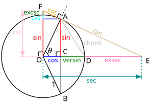


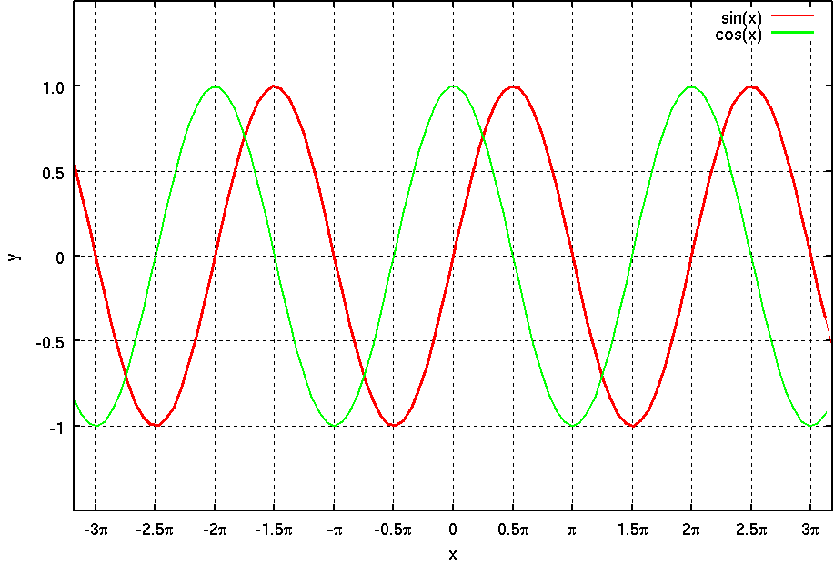


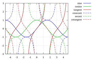
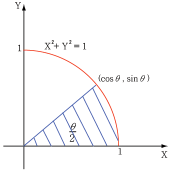
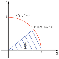

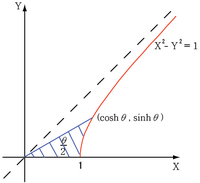


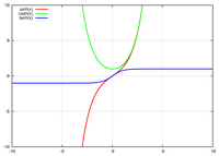
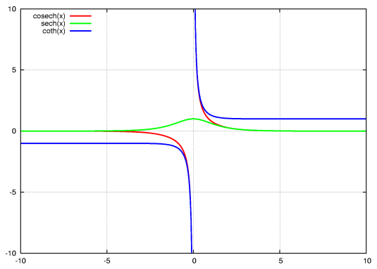
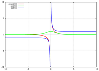


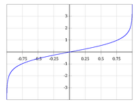
![{\displaystyle {\begin{aligned}\operatorname {arsinh} \,z&=\ln(z+{\sqrt {z^{2}+1}}\,)\\[2.5ex]\operatorname {arcosh} \,z&=\ln(z+{\sqrt {z+1}}{\sqrt {z-1}}\,)\\[1.5ex]\operatorname {artanh} \,z&={\tfrac {1}{2}}\ln \left({\frac {1+z}{1-z}}\right)\\\operatorname {arcoth} \,z&={\tfrac {1}{2}}\ln \left({\frac {z+1}{z-1}}\right)\\\operatorname {arcsch} \,z&=\ln \left({\frac {1}{z}}+{\sqrt {{\frac {1}{z^{2}}}+1}}\,\right)\\\operatorname {arsech} \,z&=\ln \left({\frac {1}{z}}+{\sqrt {{\frac {1}{z}}+1}}\,{\sqrt {{\frac {1}{z}}-1}}\,\right)\end{aligned}}}](https://services.fandom.com/mathoid-facade/v1/media/math/render/svg/c73155c895a399ca6d96aed4eee53e21671a2e05)

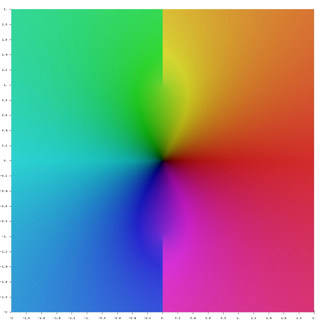

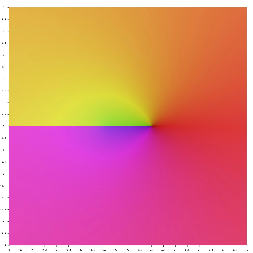

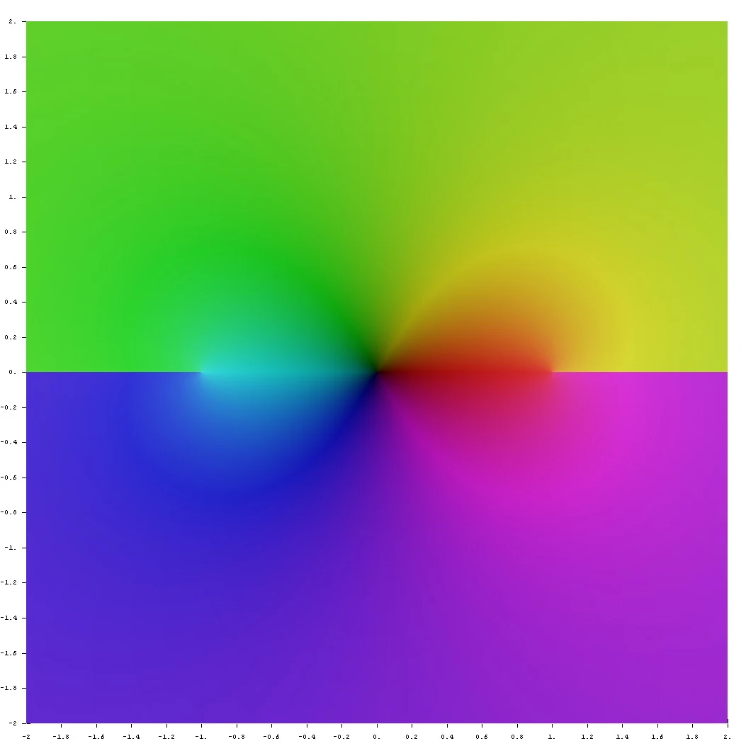

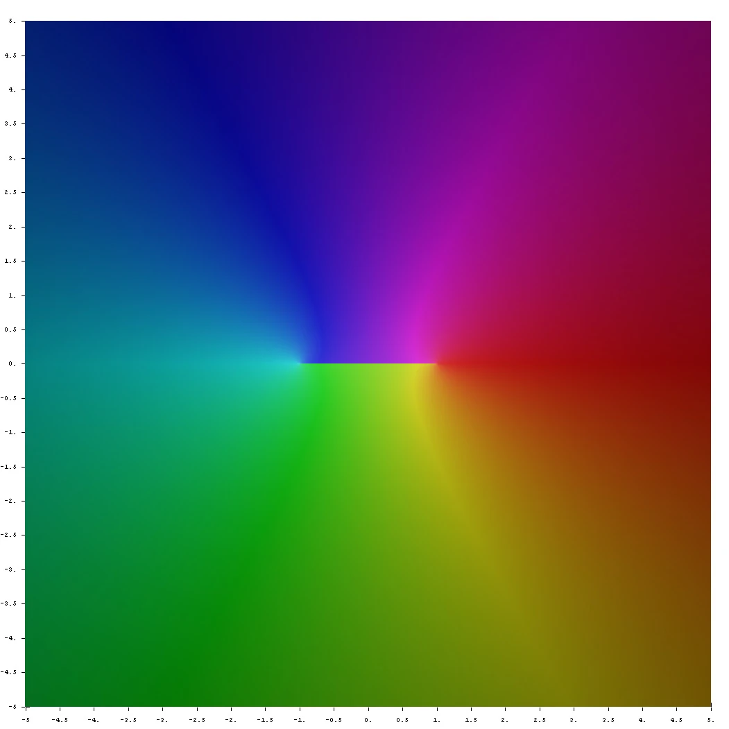

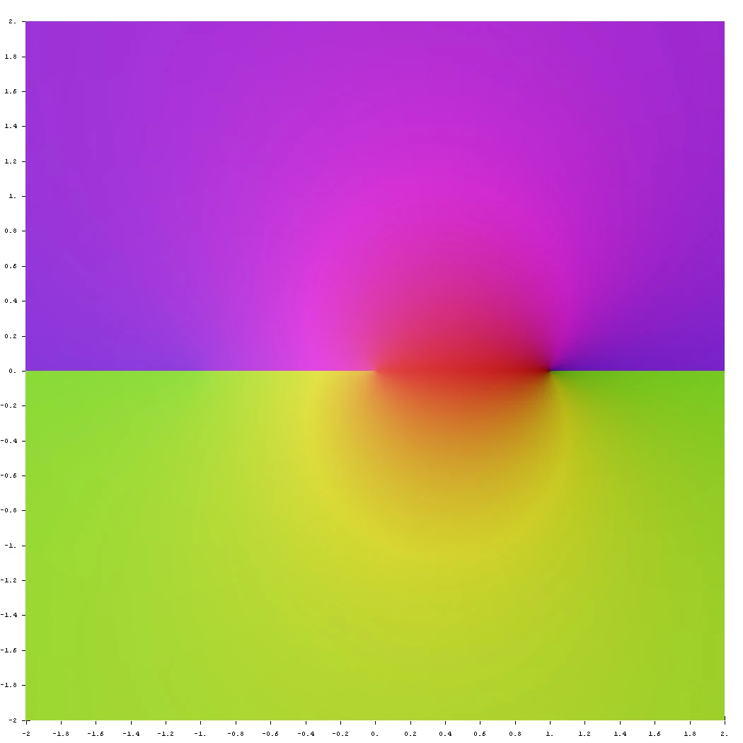

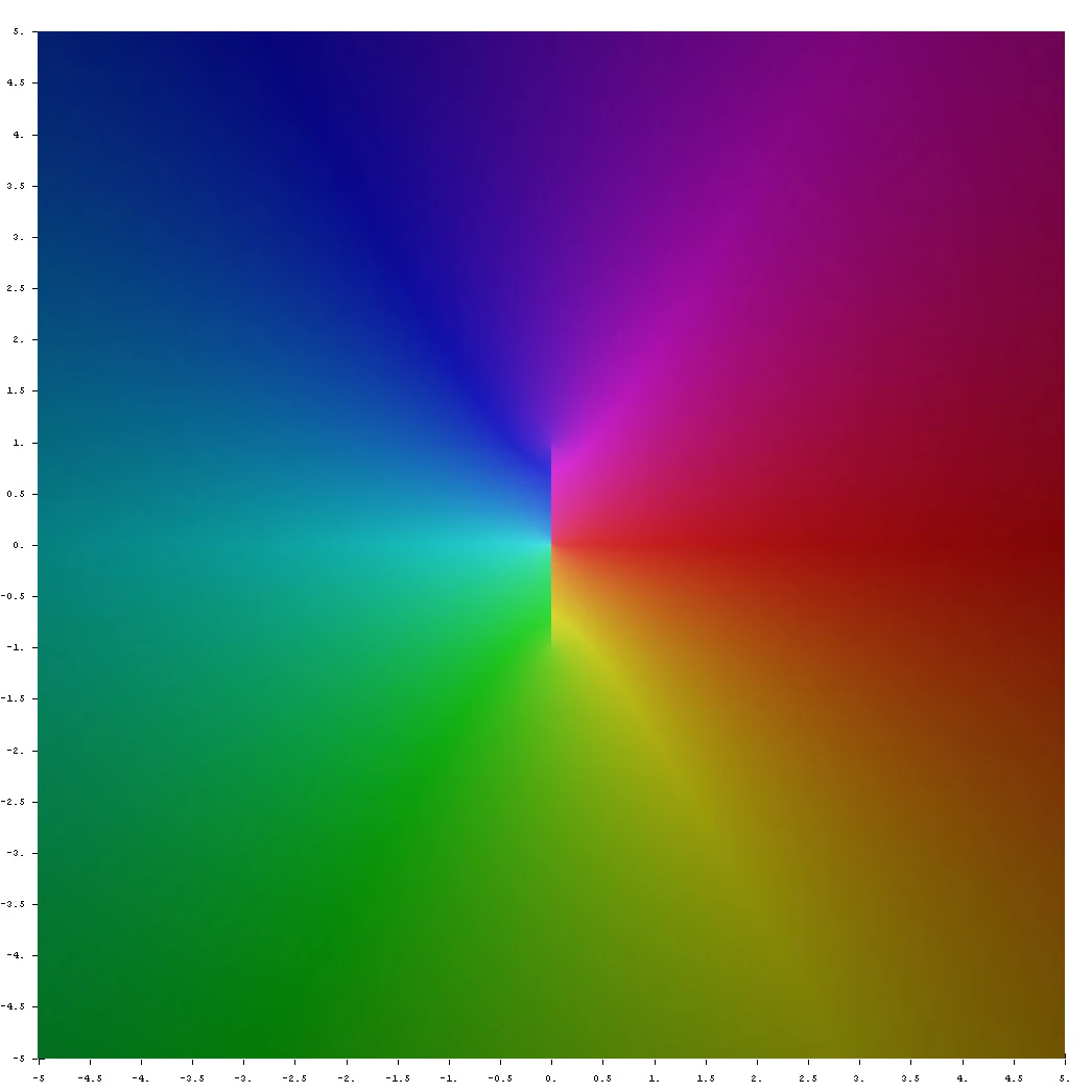


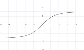
![{\displaystyle {\begin{aligned}{\rm {gd}}\,x&=\int _{0}^{x}{\frac {dt}{\cosh t}}\\[8pt]&=\arcsin \left(\tanh x\right)=\mathrm {arctan} \left(\sinh x\right)\\[8pt]&=2\arctan \left[\tanh \left({\frac {1}{2}}x\right)\right]=2\arctan(e^{x})-{\frac {1}{2}}\pi .\end{aligned}}\,\!}](https://services.fandom.com/mathoid-facade/v1/media/math/render/svg/8b058edcb10fa198ee03c4cb3fda0f0f6ed5964b)


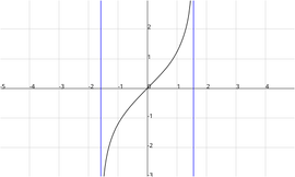

![{\displaystyle {\begin{aligned}\operatorname {gd} ^{-1}\,x&=\int _{0}^{x}{\frac {dt}{\cos t}}\\[8pt]&=\ln \left|{\frac {1+\sin x}{\cos x}}\right|={\frac {1}{2}}\ln \left|{\frac {1+\sin x}{1-\sin x}}\right|\\[8pt]&=\ln \left|\tan x+\sec x\right|=\ln \left|\tan \left({\frac {1}{4}}\pi +{\frac {1}{2}}x\right)\right|\\[8pt]&=\mathrm {artanh} \,(\sin x)=\mathrm {arsinh} \,(\tan x).\end{aligned}}}](https://services.fandom.com/mathoid-facade/v1/media/math/render/svg/6c74505b3962bda91ee6c56e01f3986a19b6a90b)

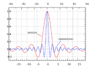


")
")
")
")


![{\displaystyle {\begin{aligned}\arcsin x&{}=-i\,\log \left(i\,x+{\sqrt {1-x^{2}}}\right)&{}=\operatorname {arccsc} {\frac {1}{x}}\\[10pt]\arccos x&{}=i\,\log \left(x-i\,{\sqrt {1-x^{2}}}\right)={\frac {\pi }{2}}\,+i\log \left(i\,x+{\sqrt {1-x^{2}}}\right)={\frac {\pi }{2}}-\arcsin x&{}=\operatorname {arcsec} {\frac {1}{x}}\\[10pt]\arctan x&{}={\frac {1}{2}}\,i\left(\log \left(1-i\,x\right)-\log \left(1+i\,x\right)\right)&{}=\operatorname {arccot} {\frac {1}{x}}\\[10pt]\operatorname {arccot} x&{}={\frac {1}{2}}\,i\left(\log \left(1-{\frac {i}{x}}\right)-\log \left(1+{\frac {i}{x}}\right)\right)&{}=\arctan {\frac {1}{x}}\\[10pt]\operatorname {arcsec} x&{}=-i\,\log \left(i\,{\sqrt {1-{\frac {1}{x^{2}}}}}+{\frac {1}{x}}\right)=i\,\log \left({\sqrt {1-{\frac {1}{x^{2}}}}}+{\frac {i}{x}}\right)+{\frac {\pi }{2}}={\frac {\pi }{2}}-\operatorname {arccsc} x&{}=\arccos {\frac {1}{x}}\\[10pt]\operatorname {arccsc} x&{}=-i\,\log \left({\sqrt {1-{\frac {1}{x^{2}}}}}+{\frac {i}{x}}\right)&{}=\arcsin {\frac {1}{x}}\end{aligned}}}](https://services.fandom.com/mathoid-facade/v1/media/math/render/svg/7db6d6767c4ce375213fd58f8c3688334f49481e)


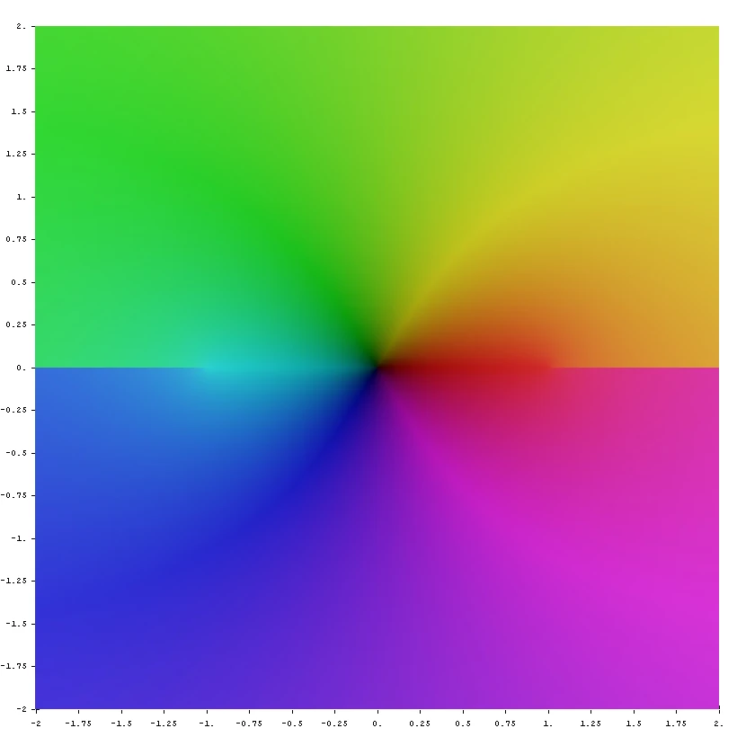
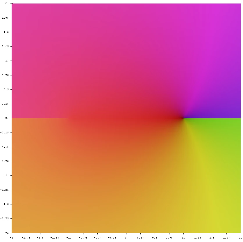
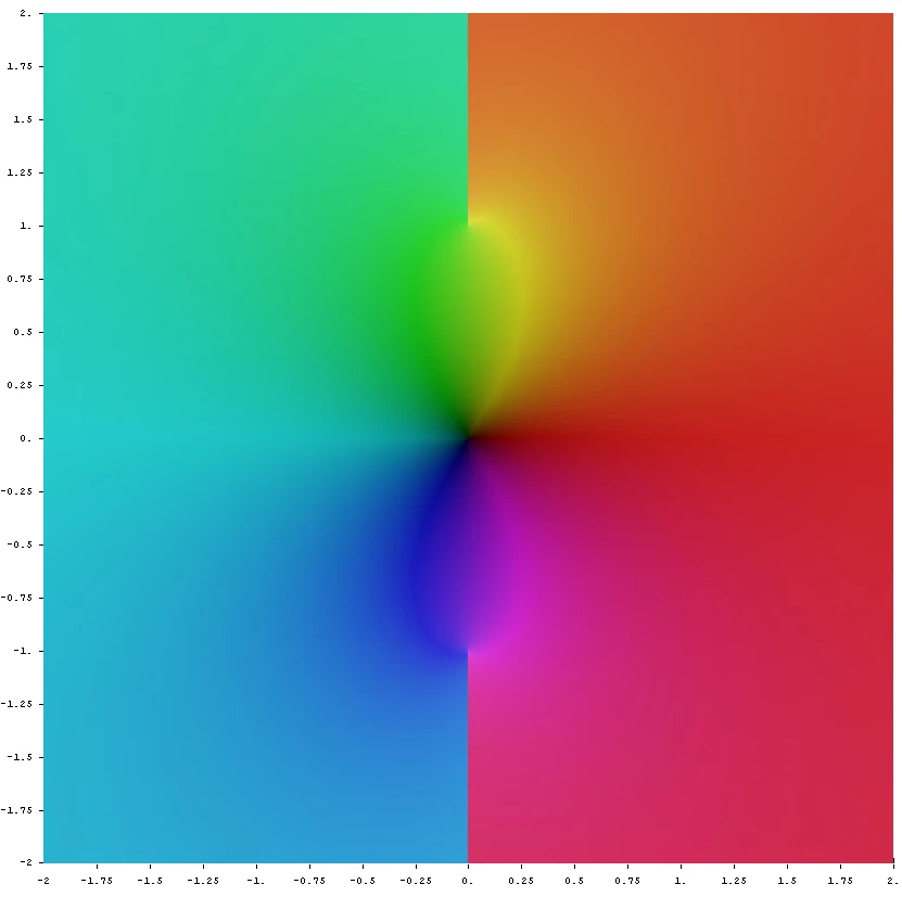
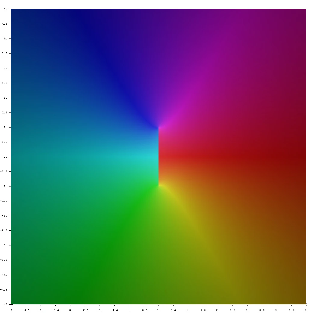
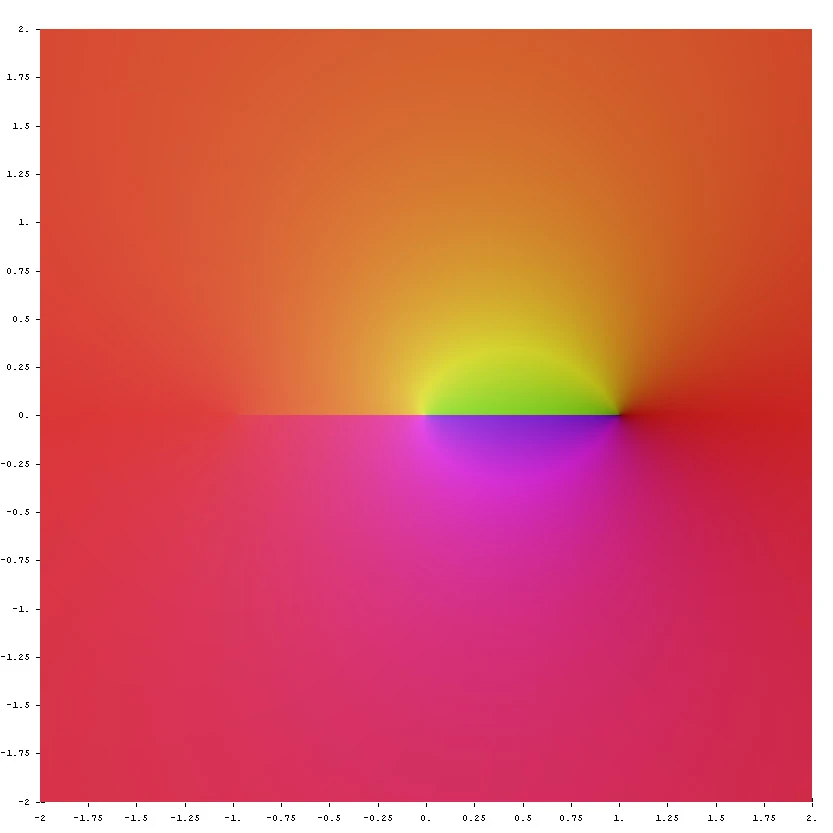
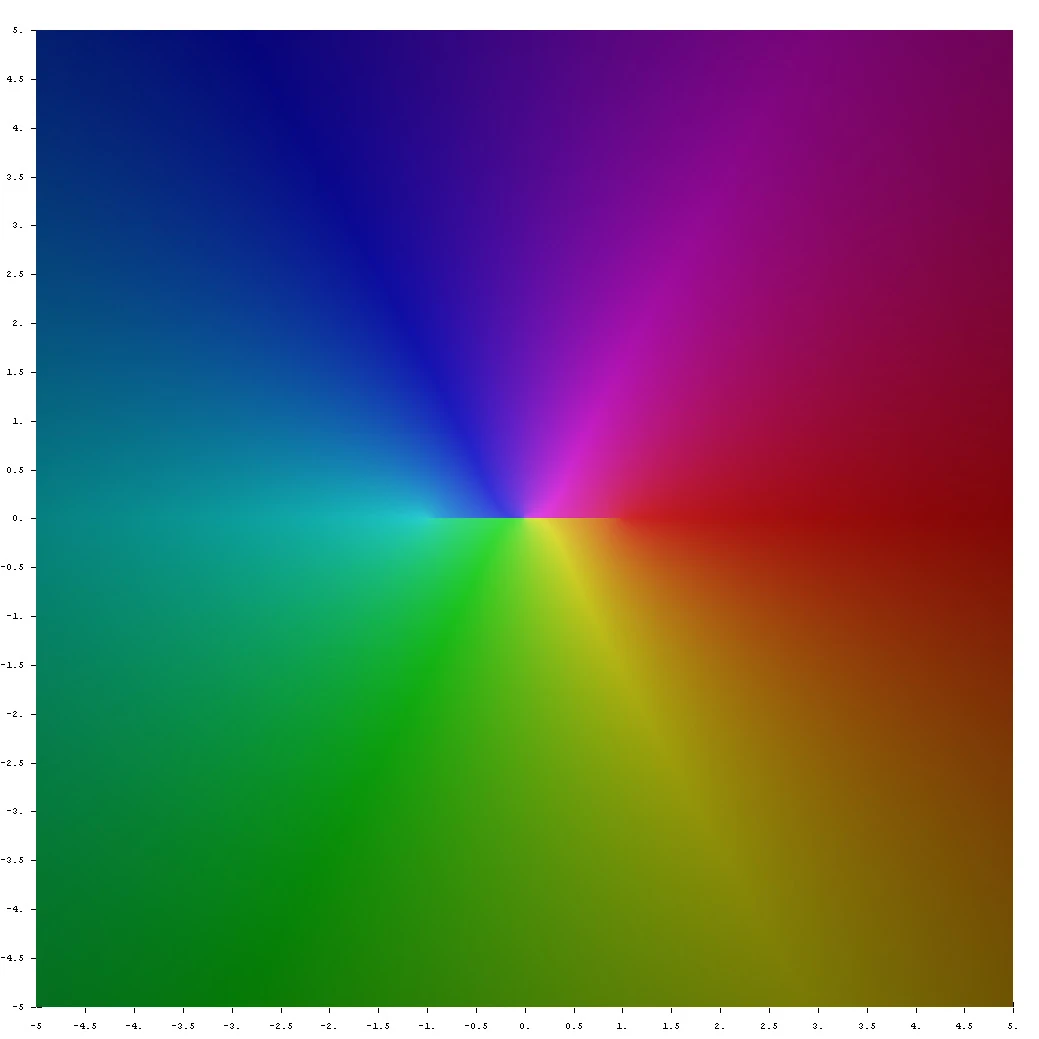


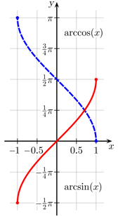

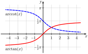

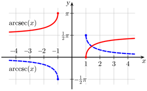


![{\displaystyle {\begin{aligned}&{}\quad \left({\begin{array}{rr}\cos \phi &-\sin \phi \\\sin \phi &\cos \phi \end{array}}\right)\left({\begin{array}{rr}\cos \theta &-\sin \theta \\\sin \theta &\cos \theta \end{array}}\right)\\[12pt]&=\left({\begin{array}{rr}\cos \phi \cos \theta -\sin \phi \sin \theta &-\cos \phi \sin \theta -\sin \phi \cos \theta \\\sin \phi \cos \theta +\cos \phi \sin \theta &-\sin \phi \sin \theta +\cos \phi \cos \theta \end{array}}\right)\\[12pt]&=\left({\begin{array}{rr}\cos(\theta +\phi )&-\sin(\theta +\phi )\\\sin(\theta +\phi )&\cos(\theta +\phi )\end{array}}\right)\end{aligned}}}](https://services.fandom.com/mathoid-facade/v1/media/math/render/svg/48573fd9c5b38b4b6f0d1fdc320f3ef8cb225f68)


![{\displaystyle {\begin{aligned}e_{0}&=1\\[6pt]e_{1}&=\sum _{1\leq i\leq n}x_{i}&&=\sum _{1\leq i\leq n}\tan \theta _{i}\\[6pt]e_{2}&=\sum _{1\leq i<j\leq n}x_{i}x_{j}&&=\sum _{1\leq i<j\leq n}\tan \theta _{i}\tan \theta _{j}\\[6pt]e_{3}&=\sum _{1\leq i<j<k\leq n}x_{i}x_{j}x_{k}&&=\sum _{1\leq i<j<k\leq n}\tan \theta _{i}\tan \theta _{j}\tan \theta _{k}\\&{}\ \ \vdots &&{}\ \ \vdots \end{aligned}}}](https://services.fandom.com/mathoid-facade/v1/media/math/render/svg/12f5fca7f9673a6dea28ca47f245514d457d72e6)


![{\displaystyle {\begin{aligned}\sec(\theta _{1}+\cdots +\theta _{n})&={\frac {\sec \theta _{1}\cdots \sec \theta _{n}}{e_{0}-e_{2}+e_{4}-\cdots }}\\[8pt]\csc(\theta _{1}+\cdots +\theta _{n})&={\frac {\sec \theta _{1}\cdots \sec \theta _{n}}{e_{1}-e_{3}+e_{5}-\cdots }}\end{aligned}}}](https://services.fandom.com/mathoid-facade/v1/media/math/render/svg/994f0b19b1359dd0f14d1332e69d6b1fd730da70)
![{\displaystyle {\begin{aligned}\sec(\alpha +\beta +\gamma )&={\frac {\sec \alpha \sec \beta \sec \gamma }{1-\tan \alpha \tan \beta -\tan \alpha \tan \gamma -\tan \beta \tan \gamma }}\\[8pt]\csc(\alpha +\beta +\gamma )&={\frac {\sec \alpha \sec \beta \sec \gamma }{\tan \alpha +\tan \beta +\tan \gamma -\tan \alpha \tan \beta \tan \gamma }}\end{aligned}}}](https://services.fandom.com/mathoid-facade/v1/media/math/render/svg/3dfe426772394b9ffaac25190ff5bd7bd18039ab)


![{\displaystyle {\begin{aligned}\tan {\frac {\theta }{2}}&=\csc \theta -\cot \theta \\&=\pm \,{\sqrt {1-\cos \theta \over 1+\cos \theta }}\\[8pt]&={\frac {\sin \theta }{1+\cos \theta }}\\[8pt]&={\frac {1-\cos \theta }{\sin \theta }}\\[10pt]\tan {\frac {\eta +\theta }{2}}&={\frac {\sin \eta +\sin \theta }{\cos \eta +\cos \theta }}\\[8pt]\tan \left({\frac {\theta }{2}}+{\frac {\pi }{4}}\right)&=\sec \theta +\tan \theta \\[8pt]{\sqrt {\frac {1-\sin \theta }{1+\sin \theta }}}&={\frac {1-\tan(\theta /2)}{1+\tan(\theta /2)}}\end{aligned}}}](https://services.fandom.com/mathoid-facade/v1/media/math/render/svg/c9f3f10e417970d16e6335e40d2f440cdc8574f3)
![{\displaystyle {\begin{aligned}\cot {\frac {\theta }{2}}&=\csc \theta +\cot \theta \\&=\pm \,{\sqrt {1+\cos \theta \over 1-\cos \theta }}\\[8pt]&={\frac {\sin \theta }{1-\cos \theta }}\\[8pt]&={\frac {1+\cos \theta }{\sin \theta }}\end{aligned}}}](https://services.fandom.com/mathoid-facade/v1/media/math/render/svg/eda775f7cd44bae3698d99598a8bdf951f7fdc71)


![{\displaystyle {\begin{aligned}&\cos \left({\frac {2\pi }{21}}\right)+\cos \left(2\cdot {\frac {2\pi }{21}}\right)+\cos \left(4\cdot {\frac {2\pi }{21}}\right)\\[10pt]&{}\qquad {}+\cos \left(5\cdot {\frac {2\pi }{21}}\right)+\cos \left(8\cdot {\frac {2\pi }{21}}\right)+\cos \left(10\cdot {\frac {2\pi }{21}}\right)={\frac {1}{2}}.\end{aligned}}}](https://services.fandom.com/mathoid-facade/v1/media/math/render/svg/ec48155f844547f6dc3cfb2c7e24032cca3eb8fc)


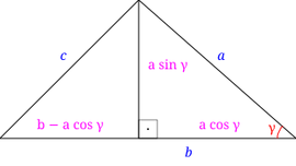


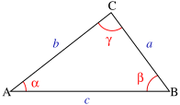
![{\displaystyle {\frac {a-b}{a+b}}={\frac {\tan[{\frac {1}{2}}(\alpha -\beta )]}{\tan[{\frac {1}{2}}(\alpha +\beta )]}}.}](https://services.fandom.com/mathoid-facade/v1/media/math/render/svg/52e4ca5157d14c994fdba1d4d48d7e6e1dec52ef)


![{\displaystyle {\frac {a-b}{a+b}}={\frac {2\sin {\tfrac {1}{2}}\left(\alpha -\beta \right)\cos {\tfrac {1}{2}}\left(\alpha +\beta \right)}{2\sin {\tfrac {1}{2}}\left(\alpha +\beta \right)\cos {\tfrac {1}{2}}\left(\alpha -\beta \right)}}={\frac {\tan[{\frac {1}{2}}(\alpha -\beta )]}{\tan[{\frac {1}{2}}(\alpha +\beta )]}}.\qquad \blacksquare }](https://services.fandom.com/mathoid-facade/v1/media/math/render/svg/79137c1b095644faf2ac799da38c41a7f12c5592)


![{\displaystyle \tan[{\frac {1}{2}}(\alpha -\beta )]={\frac {a-b}{a+b}}\tan[{\frac {1}{2}}(\alpha +\beta )]={\frac {a-b}{a+b}}\cot[{\frac {\gamma }{2}}]}](https://services.fandom.com/mathoid-facade/v1/media/math/render/svg/7ee482502d3ff54e54bf70b4bf3cf0778811cfea)


.svg)